
Indicator RBF Interpolants
An indicator RBF interpolant is a useful way of creating a region of interest in which further processing can be carried out. For example, you can use an indicator RBF interpolant to define a volume that encloses the values that are likely to be above a cut-off threshold and then use the volume as a boundary or domain to carry out further processing inside that volume. Or you might use the indicator RBF interpolant to temper the effects of extreme high-grade samples combined with sparse drilling; as all the samples are converted into either 0s or 1s, the resulting volume produced tends to be more conservative with fewer ‘blow-outs’.
Any small, uneconomic volumes that are the result of the indicator interpolant process can be automatically removed using a minimum volume filter, and a statistics tab provides detailed statistics on how the model overlaps with other data in the project.
The rest of this topic describes how to create and modify indicator RBF interpolants. It is divided into:
- Creating an Indicator RBF Interpolant
- The Indicator RBF Interpolant in the Project Tree
- Indicator RBF Interpolant Display
- Indicator RBF Interpolant Statistics
- Editing an Indicator RBF Interpolant
Creating an Indicator RBF Interpolant
To create an indicator RBF interpolant, right-click on the Numeric Models folder and select New Indicator RBF Interpolant. The New Indicator RBF Interpolant window will be displayed:
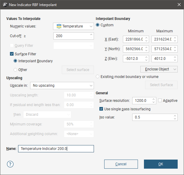
The New Indicator RBF Interpolant window is a simpler version of the Edit Indicator RBF Interpolant window. While the Numeric values object selected when the interpolant is created cannot be changed later, all the other settings, and more, can be modified. The edit window also has features to assist value selection, such as a histogram to aid selecting a cut off value. If you are unsure of any setting, accepting the default value Leapfrog Energy proposes is a good option for creating a first-pass indicator interpolant. You can then modify the values in the edit window as you iterate to improve the model.
This window is divided into four parts in which you select the values used to create the interpolant, the interpolant boundary, any compositing options and general interpolant properties.
Selecting the Values Used
In the Values To Interpolate part of the New Indicator RBF Interpolant window, select the values that will be used and choose whether or not to filter the data and use a subset of those values in the interpolant.
You can build an indicator RBF interpolant from either:
- Numeric data contained in imported drilling data.
- Points data imported into the Points folder.
All suitable data in the project is available from the Numeric values list.
You cannot change the Values To Interpolate setting once the interpolant has been created.
Setting the Cut Off
The Cut-off value will be used to generate sample points and create two output volumes:
- An Inside volume that encloses all values likely to be above or equal to the Cut-off value.
- An Outside volume that enclose all values likely to be below the Cut-off value.
The probability that the enclosing volume encloses values above the cut-off is set by the Iso value.
If you are unsure of what Cut-off value to use, you can view statistics on the distribution of the data and change the Cut-off value once the interpolant has been created. Double-click on the indicator RBF interpolant in the Numeric Models folder to open the Edit Indicator RBF Interpolant window and switch to the Cut-off tab.
You can also change the names of the Inside and Outside volumes once the interpolant has been created.
Applying a Query Filter
If you have defined a query filter and wish to use it to create the interpolant, select the filter from the Query filter list. Once the model has been created, you can remove the filter or select a different filter.
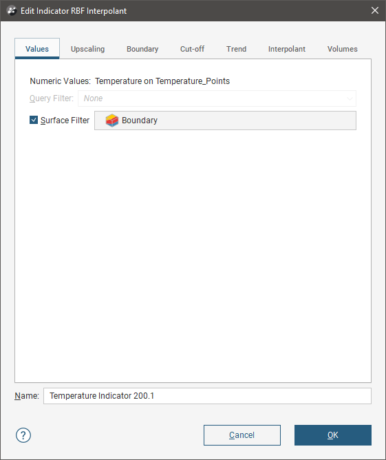
Applying a Surface Filter
All available data can be used to generate the interpolant or the data can be filtered so that only the data that is within the interpolant boundary or another boundary in the project influences the interpolant. The Surface Filter option is enabled by default, but if you wish to use all data in the project, untick the box for Surface Filter. Otherwise, you can select the Interpolant Boundary or another boundary in the project.
You can use both the Query Filter option and the Surface Filter option together.
The Interpolant Boundary
There are several ways to set the Interpolant Boundary:
- Enter values to set a Custom boundary.
- Use the controls in the scene to set the Custom boundary dimensions.
- Select another object in the project from the Enclose Object list, which could be the numeric values object being interpolated. The extents for that object will be used as the basis for the Custom boundary dimensions.
- Select another object in the project to use as the Interpolant Boundary. Click the Existing model boundary or volume option and select the required object from the list.
Once the interpolant has been created, you can further modify its boundary. See Modifying an RBF Interpolant’s Boundary With Lateral Extents and Adjusting the Interpolant Boundary in the RBF Interpolants topic for more information.
Compositing Options
When numeric values from drilling data are used to create an interpolant, there are two approaches to compositing that data:
- Composite the drilling data, then use the composited values to create an interpolant. If you select composited values to create an interpolant, compositing options will be disabled when you first create the interpolant and there will be no Compositing tab when you edit the interpolant.
- Use drilling data that hasn’t been composited to create an interpolant, then apply compositing settings to the interpolated values. If you are interpolating values that have not been composited and do not have specific Compositing values in mind, you may wish to leave this option blank as it can be changed once the model has been created. You can also change whether or not you use compositing once the interpolant has been created in the interpolant’s Compositing tab.
If you are interpolating points, compositing options will be disabled.
See Numeric Composites for more information on the effects of the Compositing length, For end lengths less than, Minimum coverage and Additional weighting column settings.
General Interpolant Properties
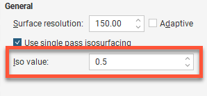
Set the Surface resolution for the interpolant, whether or not the resolution is adaptive and whether or not the interpolant uses single-pass isosurfacing. See Surface Resolution in Leapfrog Energy for more information on the effects of these settings. The resolution can be changed once the interpolant has been created, so setting a value in the New Indicator RBF Interpolant window is not vital. A lower value will produce more detail, but calculations will take longer.
An indicator RBF interpolant produces a single isosurface that is used to determine the likelihood of values falling inside or outside of the cut-off threshold. The Iso value can be set to values from 0.1 to 0.9. Clicking the arrows changes the Iso value in steps of 0.1. To use a different value, enter it from the keyboard. Again, this option can be changed once the interpolant has been created, with the added assistance of a values histogram. Double-click on the indicator RBF interpolant in the Numeric Models folder to open the Edit Indicator RBF Interpolant window and switch to the Cut-off tab.
Enter a Name for the new interpolant and click OK.
Once you have created an interpolant, you can adjust its properties by double-clicking on it. You can also double-click on the individual objects that make up the interpolant.
See also:
- Copying a Numeric Model
- Creating a Static Copy of a Numeric Model
- Exporting Numeric Model Volumes and Surfaces
The Indicator RBF Interpolant in the Project Tree
The new interpolant will be created and added to the Numeric Models folder. The new interpolant contains other objects that represent different parts of the interpolant:
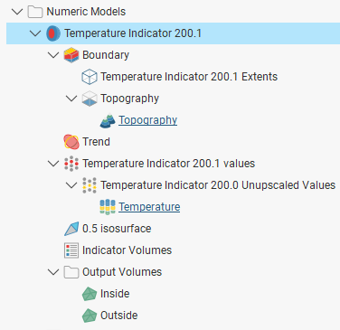
- The Boundary object defines the limits of the interpolant. See Adjusting the Interpolant Boundary.
- The Trend object describes the trend applied in the interpolant. See Changing the Trend for an Indicator RBF Interpolant.
- The sample grouping object (
 ) is the inside/outside sample grouping, which is generated by backflagging the indicator calculations on the values used. See Adjusting the Values Used for information on changing settings relating to how the sample points are grouped.
 - The isosurface is set to the specified Iso value.
- The Indicator Volumes legend defines the colours used to display the volumes.
- The Output Volumes folder contains the Inside and Outside volumes.
Other objects may appear in the project tree under the interpolant as you make changes to it. See Editing an Indicator RBF Interpolant below for more information on the changes you can make.
Indicator RBF Interpolant Display
Display the interpolant by:
- Dragging the interpolant into the scene
- Right-clicking on the interpolant and selecting View Output Volumes
- Right-clicking on the interpolant and selecting View Isosurfaces
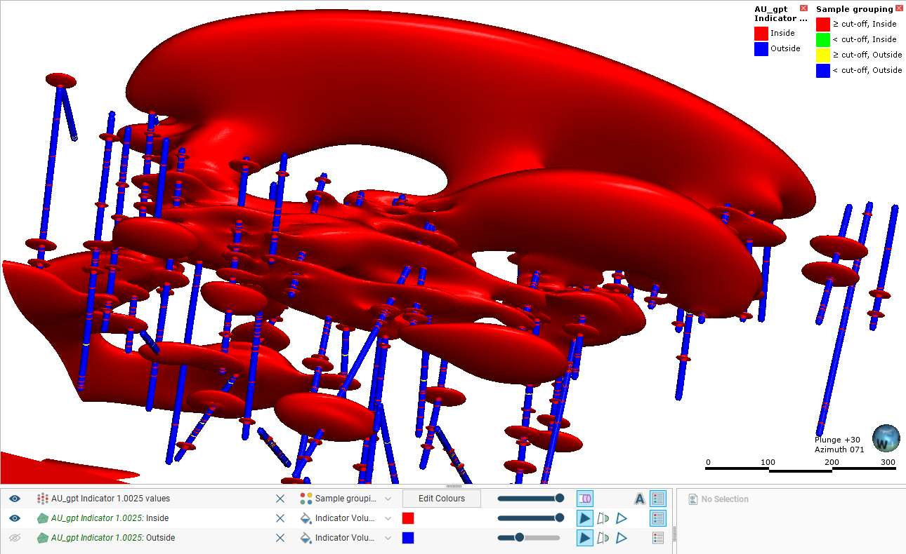
You can also display the sample grouping (![]() ) generated as part of the interpolant, which is useful in making decisions about the Cut-off value and the Iso value:
) generated as part of the interpolant, which is useful in making decisions about the Cut-off value and the Iso value:
Indicator RBF Interpolant Statistics
You can view the statistics for the indicator RBF interpolant by right-clicking on the interpolant and selecting Statistics. Use the information available to adjust the cut-off value and other interpolant properties:
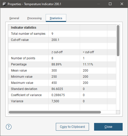
You can copy the information displayed in the Statistics tab to the clipboard for use in other applications.
Editing an Indicator RBF Interpolant
To edit an indicator RBF interpolant, you can either double-click on the interpolant in the Numeric Models folder or right-click and select Open. The window that appears is divided into tabs that let you change the different objects that make up the interpolant. Many of the options are the same as those for RBF and multi-domained RBF interpolants.
When creating an indicator RBF interpolant, only a basic set of parameters is used. The Edit Indicator RBF Interpolant windows provide finer controls over these basic parameters so you can refine the interpolant to factor in real-world observations and account for limitations in the data.
- Adjusting the Values Used
- Compositing Parameters for an Indicator RBF Interpolant
- Adjusting the Interpolant Boundary
- The Cut-Off Value
- Changing the Trend for an Indicator RBF Interpolant
- Adjusting Interpolation Parameters
- Indicator RBF Interpolant Surfacing and Volume Options
Adjusting the Values Used
The Values tab in the Edit Indicator RBF Interpolant window shows the values used in creating the interpolant and provides options for filtering the data. You cannot change the values used, but you can filter the values using the Query filter and Surface filter options.
The sample grouping object (![]() ) in the project tree is not the values used, but is instead the inside/outside sample grouping generated by backflagging the indicator calculations on the input values (
) in the project tree is not the values used, but is instead the inside/outside sample grouping generated by backflagging the indicator calculations on the input values (![]() ). You can adjust the input values using a contour polyline or by adding points. Both options are available by expanding the interpolant in the project tree, then right-clicking on the sample grouping object (
). You can adjust the input values using a contour polyline or by adding points. Both options are available by expanding the interpolant in the project tree, then right-clicking on the sample grouping object (![]() ):
):
These options are described below in Adding a Contour Polyline and Adding Points below.
Adding a Contour Polyline
You can adjust the values using contour polylines set to inside (1), outside (0) or to the iso-value. Adding a contour polyline does not affect the indicator’s statistics.
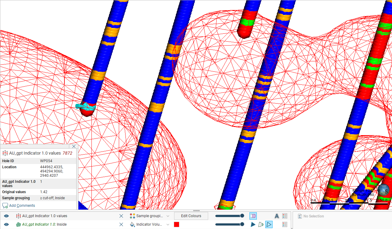
Setting a contour to inside or outside is a useful way of controlling blow-outs. Here, the inside volume occurs in the corner of the model because of the high-value points at the bottom of the well:
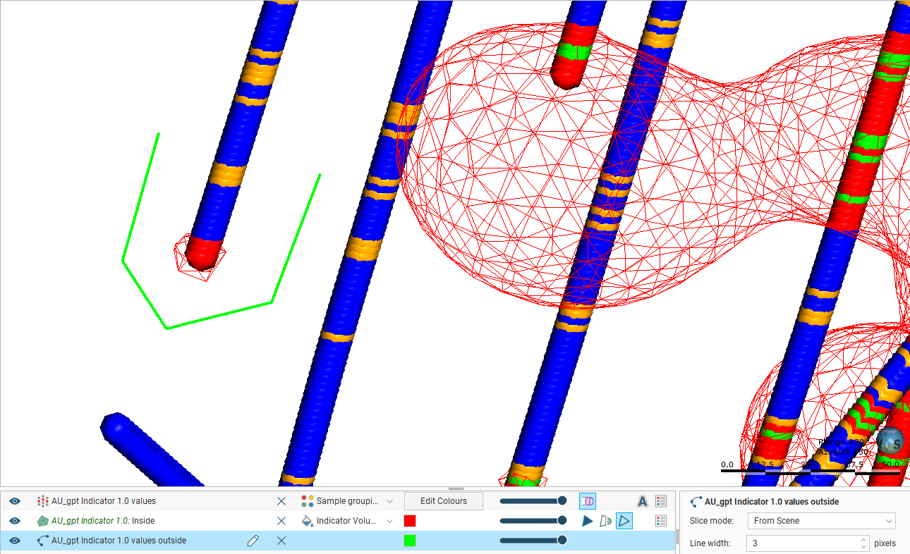
This can be adjusted by drawing a contour polyline below the bottom of the wells and setting it to the outside value. For example, adding a polyline (in green) below the bottom of well shown above removes the blow-out (the part of the mesh with only the edges shown):
Polylines must be drawn either on the slicer or on an object. Here a slicer has been drawn across the well and the scene repositioned to draw around the end of the well:
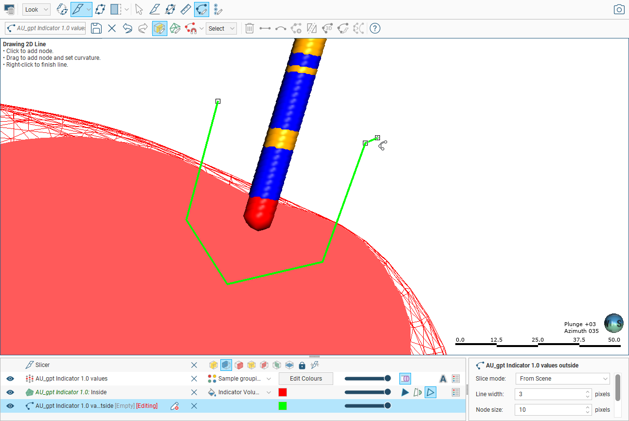
Drawing a contour polyline precisely on the well gives Leapfrog Energy conflicting data at the same location, which is why the polyline should be drawn below the well. To draw a polyline below a well without using the slicer, first draw the polyline on the well, then move its nodes so the polyline lies below the well.
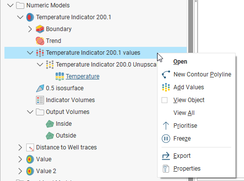
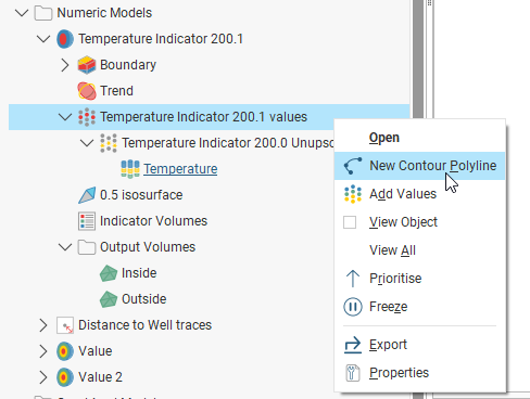
To add a contour polyline, expand the interpolant in the project tree. Right-click on the values object and select New Contour Polyline:
Next, choose whether you will draw a new polyline or use one already in the project, then select the contour value:
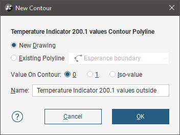
Click OK. If you have chosen the New Drawing option, the new object will be created in the project tree and drawing tools will appear in the scene. Start drawing in the scene as described in Drawing in the Scene. When you have finished drawing, click the Save button (![]() ). The new contour will automatically be added to the interpolant and will appear in the project tree as part of the interpolant’s values object.
). The new contour will automatically be added to the interpolant and will appear in the project tree as part of the interpolant’s values object.
To edit the polyline, right-click on it and select Edit Polyline or add it to the scene and click the Edit button (![]() ) in the shape list. If you wish to remove a contour polyline from the interpolant, right-click on it in the project tree and select Delete or Remove.
) in the shape list. If you wish to remove a contour polyline from the interpolant, right-click on it in the project tree and select Delete or Remove.
You cannot change the value on the contour once it has been created. You can, however, share the polyline and use it to create a new contour polyline. To do this, right-click on it in the project tree and select Share. The polyline will then be added to the Polylines folder and can be used elsewhere in the project.
Adding Points
To add points to an indicator RBF interpolant, right-click on the values object in the project tree and select Add Values. Leapfrog Energy will display a list of all suitable points objects in the project. Select an object and click OK.
A hyperlink to the points object will be added to the values object in the project tree. To remove the points object, right-click on the points object and select Remove.
Filtering Values
Query and surface filters can be changed by double-clicking on the interpolant in the project tree, then clicking on the Values tab.
Available filters will be listed in the Query Filter dropdown, building the indicator RBF interpolant from a subset of the available values data.
The Surface filter is enabled by default, with the default selection being the indicator RBF interpolant boundary. You can disable the surface filter to use all the data available, or you can select a different volume from the dropdown list to constrain the data influencing the indicator RBF interpolant. To modify the interpolant’s own boundary, switch to the Boundary tab.
Compositing Parameters for an Indicator RBF Interpolant
When an indicator RBF interpolant has been created from values that have not been composited, compositing parameters can be changed by double-clicking on the interpolant in the project tree, then clicking on the Compositing tab.
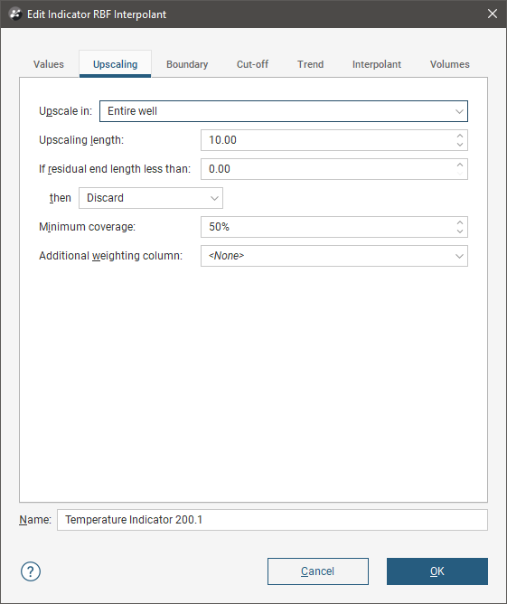
The Compositing tab will only appear for interpolants created from drilling data that has not been composited.
You can composite in the entire well or only where the data falls inside the interpolant boundary. See Numeric Composites for more information on the effects of the Compositing length, For end lengths less than and Minimum coverage settings.
Adjusting the Interpolant Boundary
To change an indicator RBF interpolant’s boundary, double-click on the interpolant in the project tree, then click on the Boundary tab:
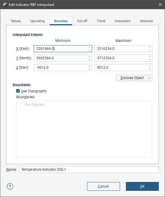
Controls to adjust the boundary will also appear in the scene.
Tick the Use Topography box to use the topography as a boundary. The topography is normally not used as a boundary for interpolants and so this option is disabled when an interpolant is first created.
The Boundaries list shows objects that have been used to modify the boundary. You can disable any of these lateral extents by unticking the box.
Techniques for creating lateral extents for indicator RBF interpolants are the same as those for RBF interpolants. See Modifying an RBF Interpolant’s Boundary With Lateral Extents for more information.
The Cut-Off Value
The Cut-off value is the value you would like to model. If you would like to visualise a shell representing values greater than 2.5, you would enter a value of 2.5 as the Cut-off value. This will be used to determine whether input values are treated as 0 or 1, waste or mineral. Another important consideration in visualising an indicator interpolant surface is the Iso value, which sets the probability you would like to maintain for the indicator interpolant isosurface. See Indicator RBF Interpolant Surfacing and Volume Options for more information.
To change the Cut-off value for an indicator RBF interpolant, double-click on the interpolant in the project tree, then click on the Cut-off tab. The tab also shows the distribution of the data used to create an indicator interpolant:
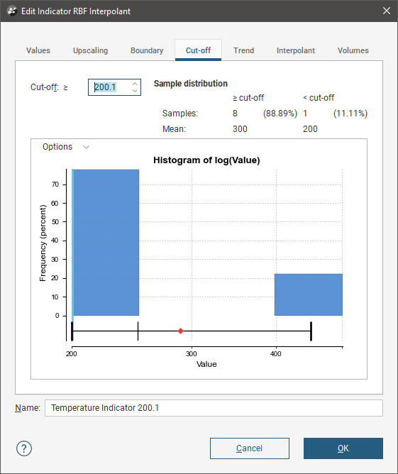
Click on the Options button to change the histogram’s display, including the Bin Width.
Adjust the Cut-off value, if required, and click OK to process the changes.
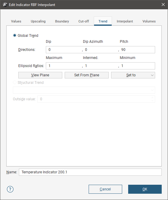
Changing the Trend for an Indicator RBF Interpolant
You can apply a global trend or a structural trend to an indicator RBF interpolant. To do this, add the interpolant to the scene, then double-click on the interpolant in the project tree. Click on the Trend tab in the Edit Indicator RBF Interpolant window.
Techniques for setting a trend for an indicator RBF interpolant are the same as those for an RBF interpolant. See Using a Global Trend and Using a Structural Trend in Changing the Trend for an RBF Interpolant.
Adjusting Interpolation Parameters
To adjust interpolation parameters for an indicator RBF interpolant, double-click on the interpolant in the project tree, then click on the Interpolant tab:
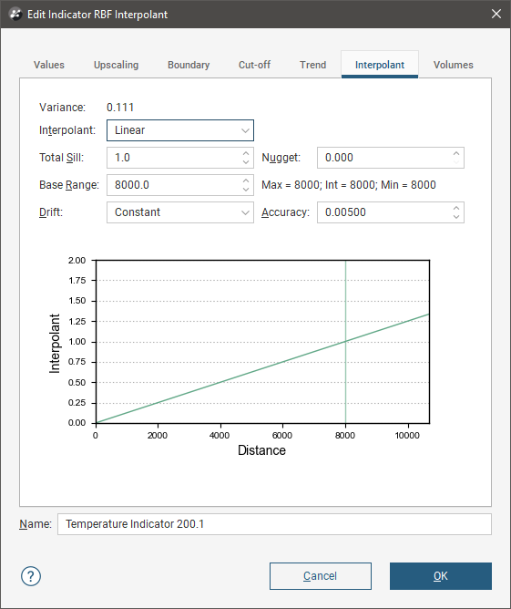
Two models are available, the spheroidal interpolant and the linear interpolant. See the Interpolant Functions topic for more information on the settings in this tab.
Indicator RBF Interpolant Surfacing and Volume Options
To change the properties of the isosurface for an indicator RBF interpolant, double-click on the interpolant in the project tree, then click on the Volumes tab:
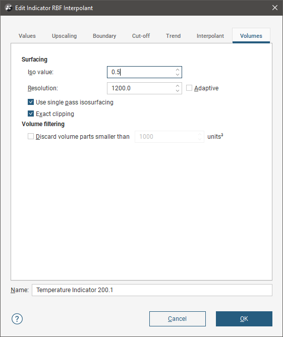
An alternative to double-clicking on the interpolant is to double-click on one of the output volumes, which opens the Edit Indicator RBF Interpolant window with the Volumes tab displayed.
The Iso value can be set to values from 0.1 to 0.9. Clicking the arrows changes the Iso value in steps of 0.1. To use a different value, enter it from the keyboard. The indicator interpolant is a probabilistic numeric model, and the Iso value is the confidence you want to use, the probability that the indicator interpolant shell contains the Cut-off value. A value of 0.1 means there is a 10% confidence, and this will result in a surface that definitely contains the mineralisation, but also will include a lot of waste. Choosing a value of 0.9 means a confidence of 90%, meaning that you almost definitely have just mineralisation inside the isosurface, depicted as a much smaller enclosing volume. However a lot of mineralisation will not be captured and will be treated as being on the ‘outside’, or waste; to achieve a confidence level of 90%, intervals are excluded that are lower probability due to high-grade material being blocked by lower grade material. Mid-range values for Iso value should therefore be preferred in most cases, rather than values at the extreme limits.
Setting a lower value for Resolution will produce more detail, but calculations can take longer. See Surface Resolution in Leapfrog Energy for more information.
When Exact clipping is enabled, the interpolant isosurface will be generated without “tags” that overhang the interpolant boundary. This setting is enabled by default when you create an interpolant.
Use Volume filtering to discard smaller parts of the volumes in which you do not wish to carry out further processing. For example, this interpolant has numerous small volumes:
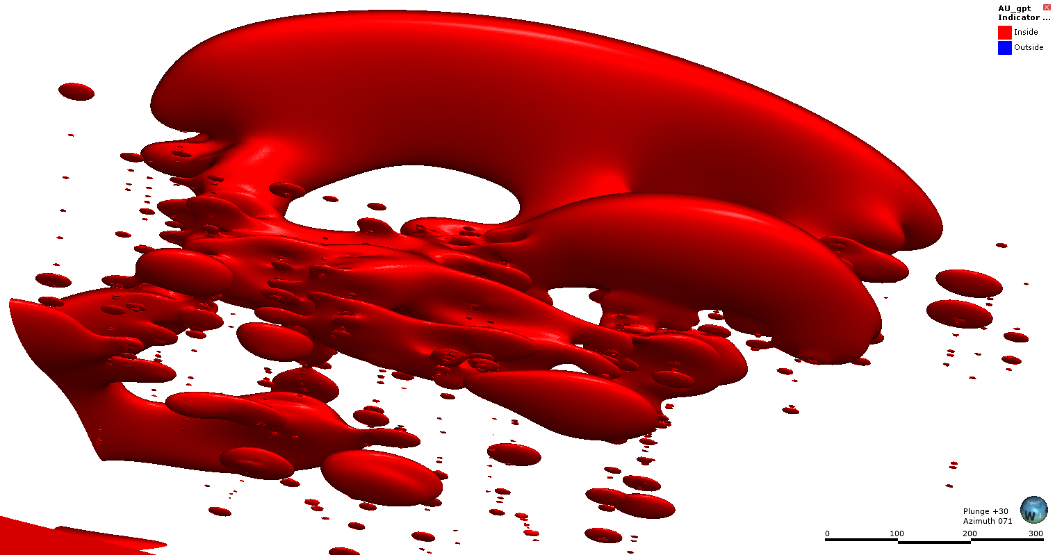
Enabling Volume filtering removes the smaller parts:

Got a question? Visit the Seequent forums or Seequent support
© 2023 Seequent, The Bentley Subsurface Company
Privacy | Terms of Use