Standard Estimators

Leapfrog Energy supports the following estimator functions:

• Inverse distance
• Nearest neighbour
• Ordinary and simple Kriging
• RBF (Radial Basis Function)

This topic describes creating and working with the different types of estimators. It is divided into:

• Copying Estimators
• Inverse Distance Estimators
• Nearest Neighbour Estimators
• Kriging Estimators
• RBF Estimators

Separate topics describe Sample Geometries (Declustering Objects) and Combined Estimators.

Copying Estimators

Estimators can be copied, which makes it easy to experiment with different parameters. Simply right-click on the estimator in the project tree and select Copy.

You can also copy one or more estimators to several other domained estimation objects at once. Select an estimator in the project tree, or select multiple estimators in the same domained estimation, right-click the selection and select Copy Estimators To from the menu. In the Copy Estimators To window, the selected estimators will appear on the left in the Source Estimators list. On the right is the Target Domained Estimations list, showing all the available domained estimations that the estimators can be copied to. Tick the box next to each domained estimation you want to receive copies of the selected estimators.

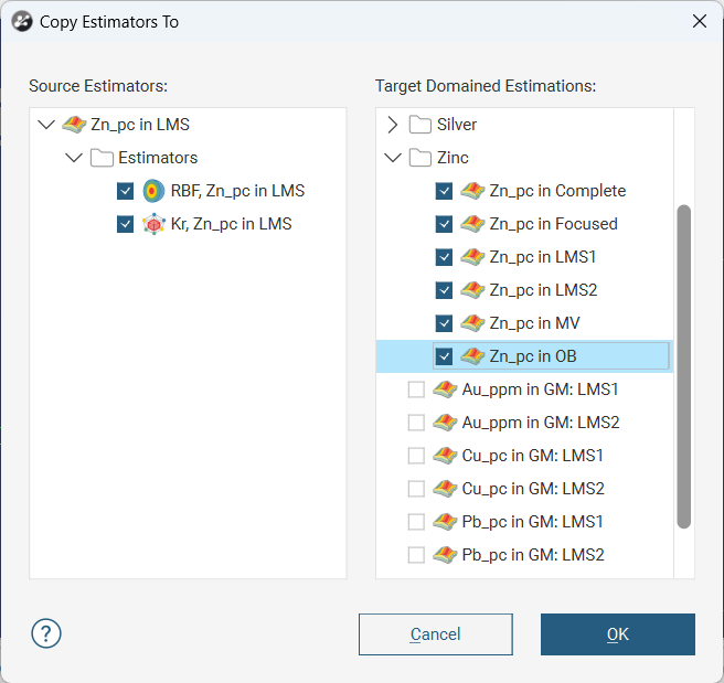
Copying of the source estimators is limited to parameters relating to the estimator itself. The following special behaviours relate to associated objects the source estimator uses:

• New copies of an estimator will reference the original estimator's variogram object; no new variogram object will be created in the destination domained estimation.
• If a source estimator's variable orientation object is a local object, the variable orientation object will be moved to the shared Variable Orientation folder under the Estimation folder in the project tree. Both the original estimator and the newly created estimators will reference the shared variable orientation object.
• If a source estimator relies upon a declustering object, the new estimators will not have any declustering object associated with them; the Declustering selection for the copied estimators will be reverted to None. A warning message will be displayed to draw attention to this. The source estimation will be unaffected.

Inverse Distance Estimators

The basic inverse distance estimator makes an estimate by an average of nearby samples weighted by their distance to the estimation point. The further a data point is from the estimate location, the less it will be relevant to the estimate and a lower weight is used when calculating the weighted mean.

To create an inverse distance estimator, right-click on the Estimators folder and select New Inverse Distance Estimator. The New Inverse Distance window will appear:

Leapfrog Energy extends the basic inverse distance function, and the inverse distance estimator supports declustering and anisotropic distance.

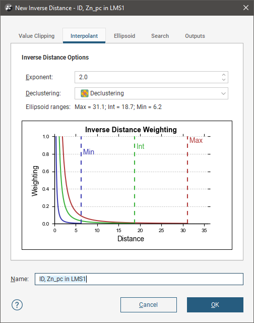
In the Interpolant tab:

• Exponent adjusts the strength of the weighting as distance increases. A higher exponent will result in a weaker weight for the same distance.
• Optionally select a Declustering object from the declustering objects defined for the domained estimation; these are saved in the Sample Geometry folder.
• Ellipsoid Ranges identify the Max, Int and Min ranges set in the Ellipsoid tab.
• A chart depicts the resultant weights that will be applied by distance.

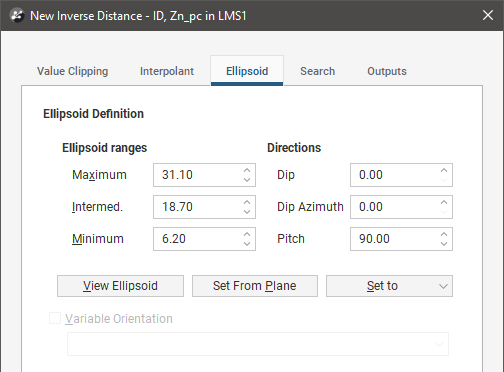
In the Ellipsoid tab:

• The Ellipsoid Definition sets the anisotropic distance and direction, scaling distances in three orthogonal directions proportionally to the range for each of the directions of the ellipsoid axes. This effectively makes the points in the direction of greater anisotropy appear closer and increases their weighting. Adjust the Ellipsoid Ranges and Directions to describe the anisotropic trend.
• Click View Ellipsoid to see an ellipsoid widget in the scene that helps to visualise the anisotropic trend.

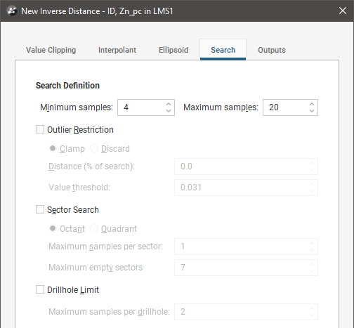
In the Search tab:

• The Minimum Samples and Maximum Samples parameters determine the number of samples required or used within the search neighbourhood.
• The remaining fields provide controls to reduce bias.
  • Outlier Restriction reduces bias by constraining the effect of high values at a distance. After ticking Outlier Restriction, you can choose to either Clamp (reduce the high value to the Value Threshold) or Discard high values that meet the criteria for outlier restrictions. It limits the samples that will be considered to those within a specified Distance percentage of the search ellipsoid size, and only those outside that distance if they are within the Value Threshold. If a sample point is beyond the Distance threshold and the point’s value exceeds the Value Threshold, it will be clamped or discarded according to the option selected.
  • Sector Search divides the search space into sectors. Choose from Octant providing eight sectors or Quadrant providing four sectors. The Maximum samples per sector threshold specifies the number of samples in a sector before more distant samples are ignored. The Maximum empty sectors threshold specifies how many sectors can have no samples before the estimator result will be set to the non-normal value without_value.
  • Well Limit constrains how many samples from the same well will be used in the search before limiting the search to the closest samples in the well and looking for samples from other wells.

In the Value Clipping tab, you can enable value clipping by ticking the Clip input values box. This caps values outside of the range set by the Lower bound and Upper bound to the bounding values.

In the Outputs tab, you can specify attributes that will be calculated when the estimator is evaluated on a block model. Value and Status attributes will always be calculated, but you can choose additional attributes that are useful to you when validating the output and reporting. These attributes are:

• The number of samples (NS) is the number of samples in the search space neighbourhood.
• The distance to the closest sample (MinD) is a cartesian (isotropic) distance rather than the ellipsoid distance.
• The average distance to sample (AvgD) is the average distance using cartesian (isotropic) distances rather than ellipsoid distances.

• The number of duplicates deleted (ND) indicates how many duplicate sample values were detected and deleted by the estimator.
• When the estimator must select from equidistant points to include or exclude in the search space because it found more samples than the Maximum Samples threshold, the number of equidistant points detected (EquiD) is recorded. You can use this output as a trigger for further investigation.

Nearest Neighbour Estimators

Nearest neighbour produces an estimate for each point by using the nearest value as a proxy for the location being estimated. There is a higher probability that the estimate for a location will be the same as the closest measured data point, than it will be for some more distance measured data point.

To create a nearest neighbour estimator, right-click on the Estimators folder and select New Nearest Neighbour Estimator. The New Nearest Neighbour window will appear:

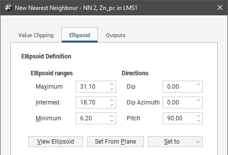
Nearest Neighbour uses an astral search algorithm to determine what point is considered the nearest. Leapfrog Energy includes support for anisotropy when determining what is considered the ‘nearest’ value. Adjust the Ellipsoid Ranges and Directions to describe the anisotropic trend.

Click View Ellipsoid to see an ellipsoid widget in the scene that helps to visualise the anisotropic trend.

In the Value Clipping tab, you can enable value clipping by ticking the Clip input values box. This caps values outside of the range set by the Lower bound and Upper bound to the bounding values.

In the Outputs tab, you can specify attributes that will be calculated when the estimator is evaluated on a block model. Value and Status attributes will always be calculated, but you can choose additional attributes that are useful to you when validating the output and reporting. These attributes are:

• The number of samples (NS) is the number of samples in the search space neighbourhood.
• The distance to the closest sample (MinD) is a cartesian (isotropic) distance rather than the ellipsoid distance.
• The average distance to sample (AvgD) is the average distance using cartesian (isotropic) distances rather than ellipsoid distances.

Kriging Estimators

Kriging is a well-accepted method of interpolating estimates for unknown points between measured data. Instead of the simplistic inverse distance and nearest neighbour estimates, covariances and a Gaussian process are used to produce the prediction.

To create a Kriging estimator, right-click on the Estimators folder and select New Kriging Estimator. The New Kriging window will appear:

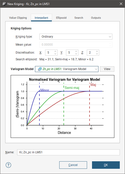
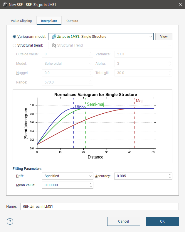
In the Interpolant tab:

• Both Ordinary and Simple Kriging are supported.
• For Simple Kriging, specify a Mean value for the local mean to use in the Kriging function.
• Discretisation sets the number of discretisation points in the X, Y and Z directions for block Kriging. Block Kriging provides a means of estimating the best value for a block instead of only at the centre of the block. Each block is broken down (discretised) into a number of sub-units without actually sub-blocking the blocks. A geologist will consider a variety of factors including spatial continuity when deciding on the discretisation to use. Set the X, Y and Z parameters to 1 for point Kriging. To use additional discretisations, copy the estimator and change the Discretisation parameters.
• Search Ellipsoid identifies the Max, Int and Min ranges set in the Ellipsoid tab.
• Select from the Variogram Model list of models defined in the Spatial Models folder.
• The View button will show an ellipsoid widget in the scene to assist in visualising the variogram model ranges and direction.
• A chart depicts colour-coded semi-variograms for the variogram model.

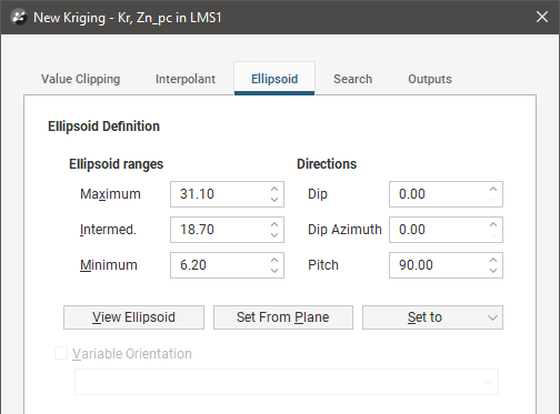
In the Ellipsoid tab:

• The Ellipsoid Definition sets the Ellipsoid Ranges and Direction.
• Click the View Ellipsoid definition to show an ellipsoid widget in the scene to assist in visualising the search ellipsoid. Note that this is not the same as the variogram model ellipsoid, unless the Set to option is used to select the variogram model to copy the details.

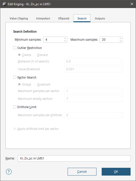
In the Search tab:

• The Minimum Samples and Maximum Samples parameters determine the number of samples required or used within the search neighbourhood.
• The remaining fields provide controls to reduce bias.
  • Outlier Restriction reduces bias by constraining the effect of high values at a distance. After ticking Outlier Restriction, you can choose to either Clamp (reduce the high value to the Value Threshold) or Discard high values that meet the criteria for outlier restrictions. It limits the samples that will be considered to those within a specified Distance percentage of the search ellipsoid size, and only those outside that distance if they are within the Value Threshold. If a sample point is beyond the Distance threshold and the point’s value exceeds the Value Threshold, it will be clamped or discarded according to the option selected.
  • Sector Search divides the search space into sectors. Choose from Octant providing eight sectors or Quadrant providing four sectors. The Maximum samples per sector threshold specifies the number of samples in a sector before more distant samples are ignored. The Maximum empty sectors threshold specifies how many sectors can have no samples before the estimator result will be set to the non-normal value without_value. When Sector Search is enabled, the translucent planes in the search ellipsoid widget change to show the search sectors.
  • Well Limit constrains how many samples from the same well will be used in the search before limiting the search to the closest samples in the well and looking for samples from other wells.

  • The Apply well limit per sector option controls the behaviour of the application of the sector search and well limits. It is only available when both Sector Search and Well Limit settings are being used. When the box is ticked, the Well Limit setting for Maximum samples per drillhole is applied per sector, so a drillhole may have more samples per drillhole than is specified in the limit, but the number is constrained to the limit for each sector the drillhole passes through. When unticked, the Well Limit setting for Maximum samples per drillhole is applied without regard to which sectors the drillhole passes through, and this may reduce the number of samples available for the search.

In the Value Clipping tab, you can enable value clipping by ticking the Clip input values box. This caps values outside of the range set by the Lower bound and Upper bound to the bounding values.

Kriging Attributes

In the Outputs tab, you can specify attributes that will be calculated when the estimator is evaluated on a block model. Value and Status attributes will always be calculated, but you can choose additional attributes that are useful to you when validating the output and reporting. These attributes are organised into two categories, Sample properties and Estimation results.

Sample properties are output attributes that relate to data sample statistics:

• The number of samples (NS) is the number of samples in the search space neighbourhood.
• The number of wells (NDh) is the number of wells used to inform the estimation, which together with number of samples can be utilised to determine if blocks are well informed or poorly informed.
• The Euclidean distance to the closest sample (MinD) is a cartesian (isotropic) distance rather than the ellipsoid distance.
• The average Euclidean distance to sample (AvgD) is the average distance using cartesian (isotropic) distances rather than ellipsoid distances.
• The anisotropic distance to the closest sample (MinAD) is the anisotropic distance used when making sample selection.
• The average anisotropic distance to sample (AvgAD) is the average anisotropic distance used when making sample selection.
• The number of duplicates deleted (ND) indicates how many duplicate sample values were detected and deleted by the estimator.

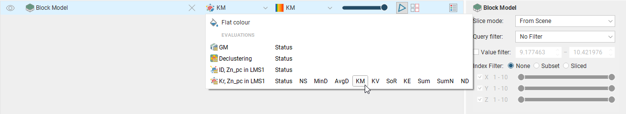
Estimation results are additional information produced by the estimation:

• Value will always be included as it is the actual estimate result.
• Status will always be included as it classifies the estimation result as a Normal result, or non-normal Blank, Without-value, Outside or Error result.
• The Kriging mean (KM) is the local mean used for the estimate based around the selected sample data. For simple Kriging, this is the specified global mean. For ordinary Kriging, it is the unknown locally constant mean that is assumed when forming the Kriging equations. This value is only dependent on the covariance function and the sample locations and values for the chosen neighbourhood. It does not depend on the evaluation volume and therefore will be the same for block Kriging and point Kriging. It can give some indication of suitability of the assumptions when doing ordinary Kriging.
• The Kriging variance (KV) is important in assessing the quality of an estimate. It grows when the covariance between the samples and the point to estimate decreases. This means that when the samples are further away from the evaluation point, the quality of the estimation decreases. For simple Kriging, the value is capped by the value of the covariance between the target volume and itself. For ordinary Kriging, higher values indicate a poor value. The Kriging variance calculation depends on whether the Variogram Model has Sill or Norm. Sill selected. Having KV based on the normalised data when Norm. Sill is selected means that KV is comparable between domains using normalised variogram models.

• The Kriging efficiency (KE) is calculated based on the block variance and Kriging variance (KV). It should be 1 when the Kriging variance is at is minimum and 0 when the Kriging variance equals the block variance.
• The slope of regression (SoR) is the slope of a linear regression of the actual value, knowing the estimated value. For simple Kriging it is 1 and for ordinary Kriging a value of 1 is desired as it indicates that the resulting estimate is conditionally unbiased. Conditional bias is to be avoided as it increases the chance that blocks will be misclassified when considering a cutoff value.
• The sum of weights (Sum) is the sum of the Kriging weights. For ordinary Kriging, the sum is constrained to being equal to 1.
• The sum of negative weights (SumN) can be used to assess the quality of an estimation. Negative weights are to be avoided or at least minimised. If there are negative weights, it is possible that the estimated value may be outside the range of the sample values. If the sum of negative weights is significantly large (when compared to the total sum), then it could result in a poorly estimated value, depending on the sample values.

When selecting the block model evaluation to display in the 3D scene, you can select either the Kriging values, or from these additional selected attributes.

RBF Estimators

The RBF estimator brings the Radial Basis Function used elsewhere in Leapfrog into estimation. Like Kriging, RBF does not use an overly-simplified method for estimating unknown points, but produces a function that models the known data and can provide an estimate for any unknown point. Where Kriging is limited to a local search neighbourhood, RBF utilises a global neighbourhood. An RBF estimator is good for grade control where there is a large amount of data.

To create an RBF estimator, right-click on the Estimators folder and select New RBF Estimator. The New RBF window will appear:

Like other estimators, a spatial model defined outside the estimator as a separate Variogram Model can be selected. The View button will show an ellipsoid widget in the scene to assist in visualising the variogram model ranges and direction.

Alternatively, in a feature unique to RBF estimators, a Structural trend can be used, if one is available in the project. Outside value provides a place to specify what value to use outside the estimation domain. What value you choose to use here will depend on the specifics of your model’s context. You may choose to set the Outside value at the long-range mean value of the data, such as using the mean from the statistics view; right-click on the numeric data object and select Statistics to find this value. Alternatively, the modelling context may call for Outside value to be set at the expected background value.

Otherwise, the RBF estimator behaves very similarly to the RBF interpolant in Leapfrog.

Drift is used to specify what the estimates should trend toward as distance increases away from data. The RBF estimator has different Drift options from the non-estimation RBF interpolants. The RBF estimator function offers the Drift options Specified and Automatic. When selecting Specified, provide a Mean Value for the trend away from data. Automatic is equivalent to the Constant option offered by non-estimation RBF interpolants, and Linear is not supported. Specified drift with a Mean Value of 0 is equivalent to None.

In the Value Clipping tab, you can enable value clipping by ticking the Clip input values box. This caps values outside of the range set by the Lower bound and Upper bound to the bounding values.

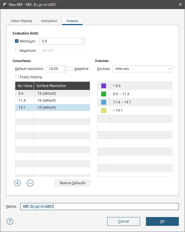
In the Outputs tab, the Minimum and MaximumEvaluation Limits constrain the values. Values outside the limits are set to either the minimum or maximum limit, as appropriate. To enable a limit, tick the checkbox and set a limit value.

In the Outputs tab, you can also define isosurfaces for an RBF estimator:

• The Default resolution will be used for all isosurfaces, unless you change the Surface Resolution setting for an individual isosurface. See Surface Resolution in Leapfrog Energy for more information on the Adaptive setting. The resolution can be changed once the estimator has been created, so setting a value in the New RBF window is not vital. A lower value will produce more detail, but calculations will take longer.
• The Volumes enclose option determines whether the volumes enclose Higher Values, Lower Values or Intervals. Again, this option can be changed once the estimator has been created.
• Click the Restore Defaults button to add a set of isosurfaces based on the estimator’s input data.
• Use the Add to add a new isosurface, then set its Iso Value.
• Click on a surface and then on the Remove button to delete any surface you do not wish to generate.