
Experimental Variogram Controls
A variogram model can be verified through the use of the experimental variography tools that use sample data. Use these to find the directions of maximum, intermediate and minimum continuity.
The rest of this topic describes the experimental variography controls in the Variogram Model window. It is divided into:
The variogram displayed in the chart is selected from the variograms listed in the panel in the top left corner of the window.
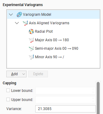
The top entry in the variograms list is the theoretical variogram model rather than an experimental variogram:
All other variograms in the list and the other controls on the left-hand side of the screen relate to Experimental Variograms.
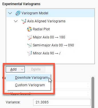
By default, there is a set of Axis Aligned Variograms. Use the Add button to add additional experimental variograms. You can add one Downhole Variogram and any number of Custom Variograms.
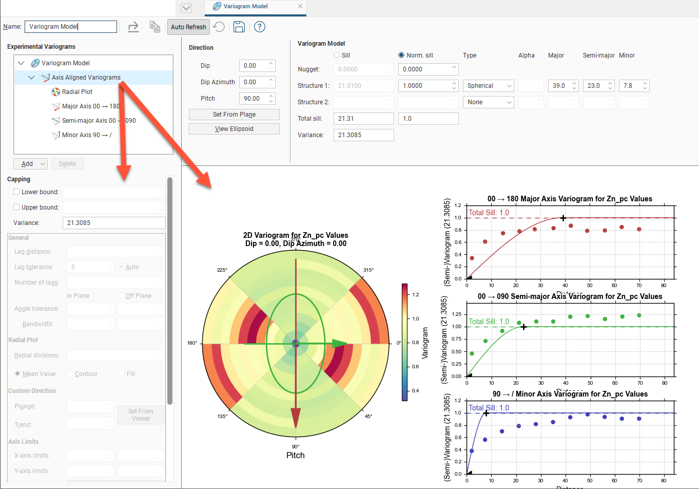
Click on one of these experimental variograms to select it and display its parameters. The displayed graph will change to match this selection. For example, here the graph and settings for the combined Axis Aligned Variograms are displayed:
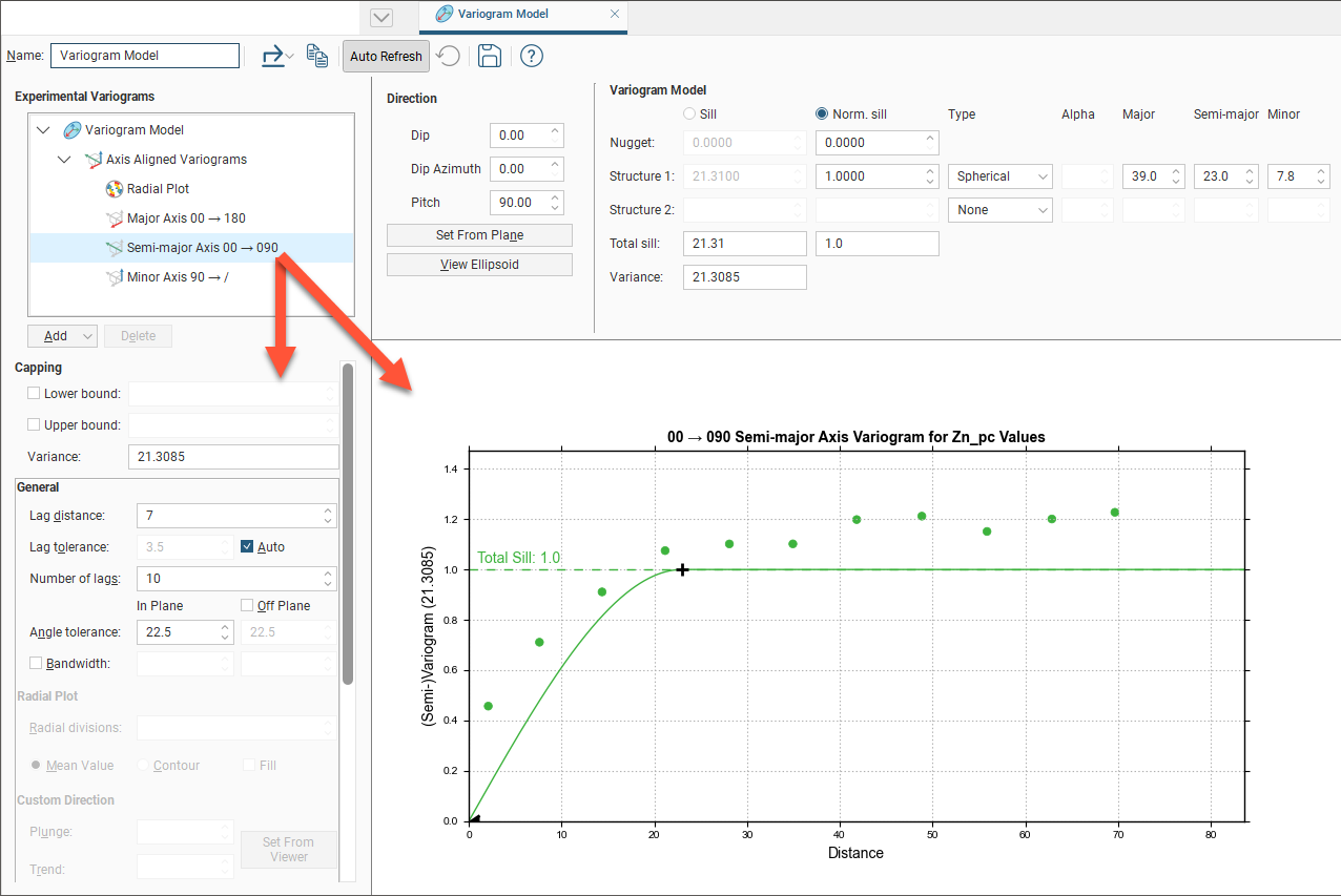
Selecting the Semi-major Axis variogram changes the chart and settings displayed:
Adjust the model variogram parameters to see the effect different parameters have when applied to the actual data.
Experimental Variogram Parameters
The experimental variogram controls along the left side of the window define the search space, define the orientation for custom variograms and change how the variograms are displayed. Some parameters are only available for some variogram types; these are discussed in later sections on each variogram type.
Capping
Data Capping fields limit the values of the Lower bound and Upper bound for the data as specified. This is not a filter that discards these points, but values below or above the caps are treated as if the value was the lower or upper bound.
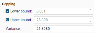
These Capping controls only affect the data values considered for the purposes of experimental variography, and they do not cap the values of the data points used in estimation. If you wish to also cap values used in estimation, set the Lower bound and Upper bound limits in the Value Clipping tab in the applicable estimator. To eliminate an anomalous data point or discard certain data values, you should modify the domain definition options using a Query Filter.
Defining the Search Space
The search space for experimental variography is not shown in the scene. It is not an ellipsoid, and should not be confused with either the variogram model ellipsoid or the estimator’s search ellipsoid.
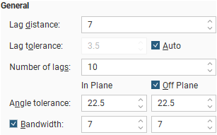
The first set of parameters controls the search space.
- Lag distance controls the size of the lag bins. The first bin will be one quarter of the size of the Lag distance. Experimental variograms generally measure lags as distances along a direction vector, though downhole variograms measure lags as distances along the wells.
- Lag tolerance allows for the reality that data pairs are rarely the same distance apart. The data is scanned and pairs are assembled after applying a Lag tolerance to the Lag distance. If the Lag tolerance Auto box is ticked, Leapfrog Energy defaults to using a Lag tolerance of half the Lag distance. Controlling the Lag tolerance explicitly allows you to test the sensitivity of the variogram. Typically, a larger value will be used for sparse data sets and a smaller value for dense data sets.
Some modelling applications treat a Lag tolerance of 0 as a special value that does not mean ‘no lag tolerance’ but instead is interpreted as meaning half the Lag distance. In Leapfrog Energy, it is possible to set Lag tolerance to 0, but this means literally what the number implies: there is no Lag tolerance and the only data pairs that are displayed are those that occur exactly at the Lag distance spacing.
- Number of lags constrains the number of lag bins in the search space.
- The In Plane and Off Plane Angle tolerance and Bandwidth settings define the search shape, and the effects of these settings are discussed in more detail below.
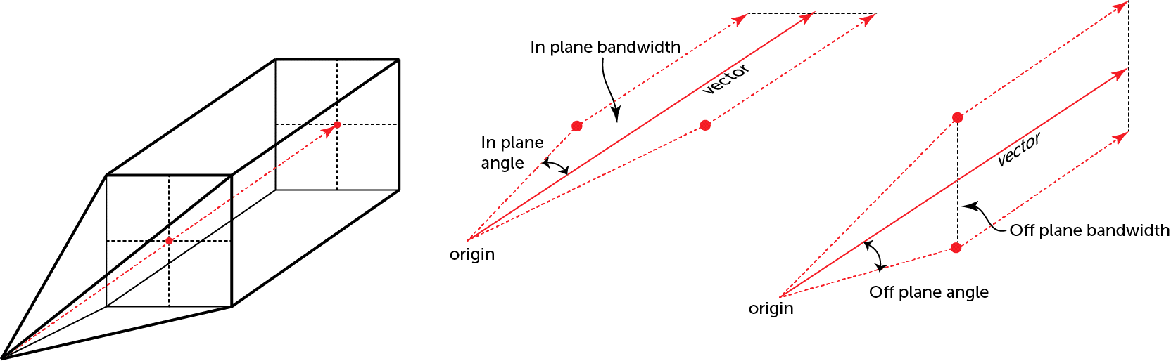
Some modelling applications describe Bandwidth as the distance measured from the vector centreline. Leapfrog Energy measures Bandwidth as the full width of the search band.
The search shape usually approximates a right rectangular pyramid on a rectangular parallelepiped. The pyramid and parallelepiped will be square if the In Plane Angle tolerance and Bandwidth are used without defining Off Plane values. Using the Off Plane Angle tolerance and Bandwidth fields will make the shape rectangular. The plane being referred to is the major-intermediate axis plane of the variogram ellipsoid, the same plane used for the radial plot. The Angle tolerance is the angle either side of a direction vector from the data point origin. Once the sides of the pyramid defined by the angle tolerances extend out to the limits specified by the Bandwidth, the search neighbourhood is constrained to the bandwidth dimensions.
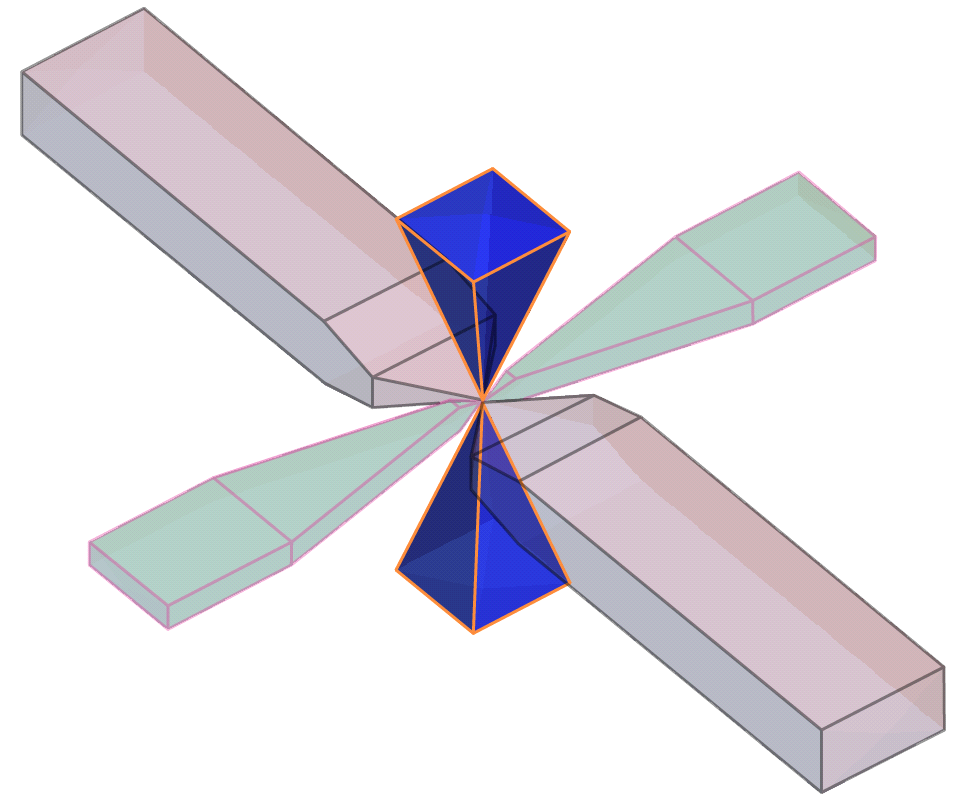
The search shape becomes a more complex “carpenter’s pencil” shape when a wide In Plane angle and a narrow Bandwidth are defined along with a narrow Off Plane angle and a wide Bandwidth, or vice versa. This rendering should assist in visualising the shape; the major axis is shown in red, the semi-major axis is shown in green, and the orthogonal minor axis in a transparent blue:
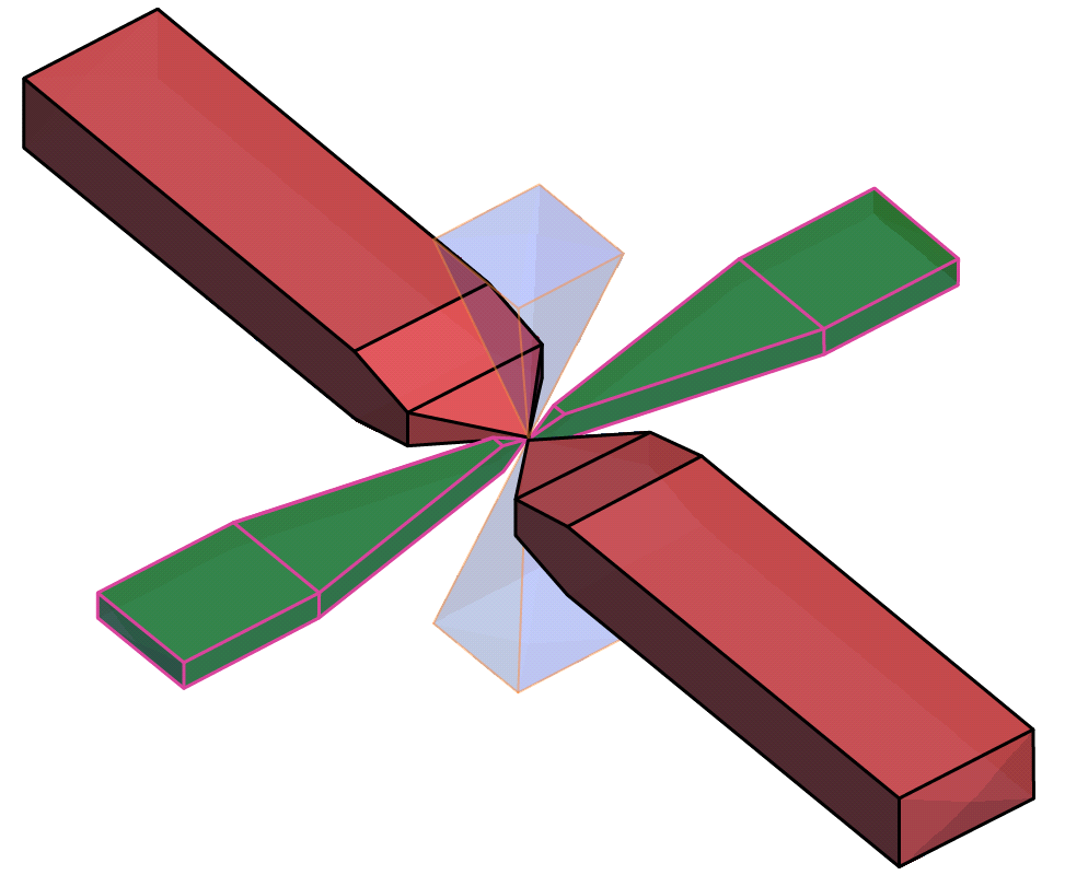
Note that although not shown here, the outer ends of the search shapes are not flat, but rounded, being defined by the surface of a sphere with a radius of the maximum distance defined by the number of lags and their size.
Off Plane Angle tolerance and Bandwidth settings cannot be set for the minor axis variogram. Because the angle tolerance and bandwidth are described relative to the major-intermediate plane and because the minor axis is orthogonal to this plane, only one angle can be described. This results in a square pyramid search shape.
The In Plane Bandwidth also cannot be set for the Minor Axis.
Note that although not shown here, the outer ends of the pyramids are rounded, defined by the surface of a sphere with a radius of the maximum distance defined by the number of lags and their size.
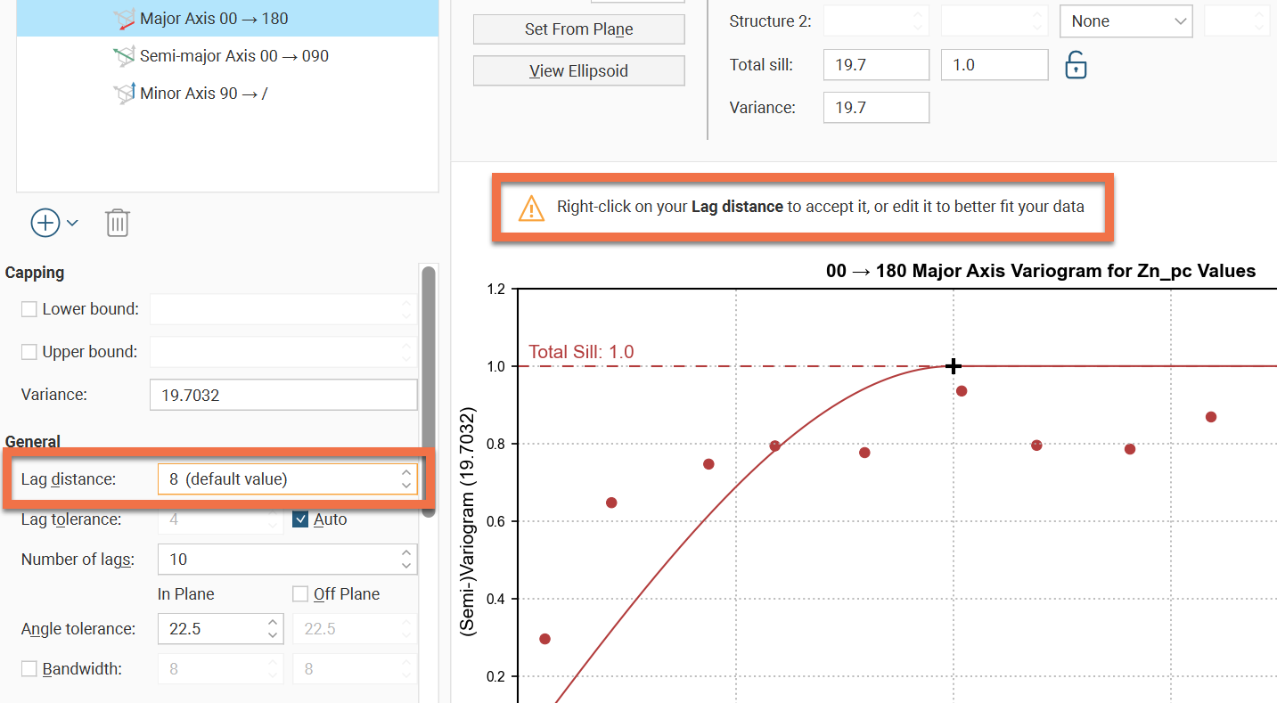
While the Lag distance field contains the unedited default value, the value is bordered in orange and a warning message appears above the chart: Right-click on your Lag distance to accept it, or edit it to better fit your data. This is a reminder that the default lag distance is not auto-fitted and a geologist’s professional judgement needs to be applied to select an appropriate value. If the value appears to be suitable, right-click on the value then select Accept Default from the pop-up menu.
Radial Plot Parameters
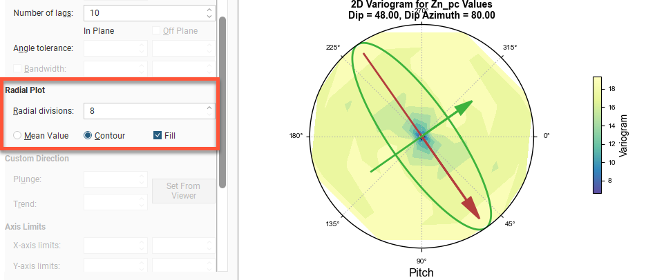
Radial Plot has parameters specifically for the radial plots in Axis Aligned Variograms.
Increasing the Radial divisions slices the space into a larger number of sectors, with each block in the radial plot covering a smaller arc of the compass. As a result, each block has a smaller volume; this also means that the amount of data in each block is reduced. Because the bandwidth angle above and below the major-intermediate plane matches the angle used to slice the plot into its sectors, increasing the Radial divisions also reduces the number of data points used above and below the plane. Using a smaller number of Radial divisions will be faster. If you increase the number of divisions, you may want to turn off Auto Refresh Graphs first and click Refresh graphs afterwards. Experiment with the number of divisions and choose the lowest number of Radial divisions that helps you gain the best understanding of continuity; this will maximise the data that falls in each division.
Mean Value will display radial plot bins coloured to indicate the mean value for each bin. Contour will display a plot showing lines of equal value. Fill shades the chart between the contour lines.
Orienting Custom Variograms
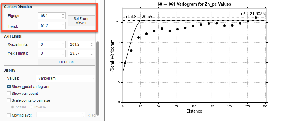
The Custom direction fields are for Custom Variograms that use the Plunge to Trend settings to orient the variogram trend. They can easily be set by orienting the scene view and then clicking the Set From Viewer button, which sets the plunge and trend to that of the scene view.
Changing Axis Limits
The Axis Limits settings control the chart scaling.
X axis limits and Y axis limits control the ranges for the X-axis and Y-axis and can effectively be used to zoom the chart. You can directly control these by manipulating the axes with your mouse. Click and drag an axis to increase or decrease the maximum limit of the axis. Right-click and drag an axis to reposition the axis so the minimum value on the axis is not zero. Double-click the axis to reset the axis minimum and maximum range to the default values. Fit Graph will auto-fit the graph to the available data.
Changing Variogram Display
The Display settings change how the variogram is displayed:
- Values offers a variety of options to plot on the chart: Variogram, Correlogram, Covariance, Relative Variogram and Pair-wise Variogram.
- Show model variogram plots the variogram on the chart.
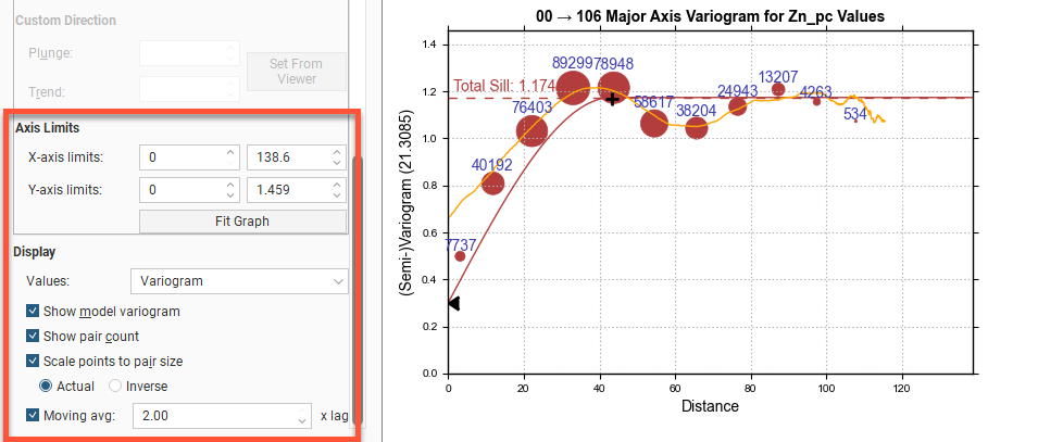
- Show pair count annotates the chart with the count of data point pairs.
- Tick the Scale points to pair size checkbox and the chart will display the plotted points with dots that scale to the size of the pair count. Choose Actual so the dots represent the pair size proportionally and Inverse to see larger dots for lower pair counts.
- Tick Moving avg for a rolling mean variogram value, drawn on the variogram plots in orange. Next to it, select a value for the window size relative to the Lag distance.The window size will be the given number times the lag distance. This window, centred on x, will be used to plot y, the average of all the variogram values falling inside the window. The lag multiplier field has a useful tooltip reminder; hover your mouse pointer over the field to see the tooltip.
The Downhole Variogram
The Downhole Variogram can be used to better define the nugget. It looks only looks at pairs of samples on the same well and uses the differences in depths to calculate the lag value.
As it isn’t associated with a specific direction, the Angle tolerance parameter is not available for the Downhole Variogram.
The Downhole Variogram chart does not plot the model variogram line; instead it shows a dotted horizontal line indicating the Total Sill and, if Sill is chosen instead of Normalised Sill, the variance.
A model is not fitted to the Downhole Variogram data because not all drillholes are oriented in the same direction. An alternative that provides a fixed direction is to use a Custom Variogram. Adjust the scene to look down a specific drillhole in the relevant direction, then choose Set From Viewer to set the Plunge to Trend values.
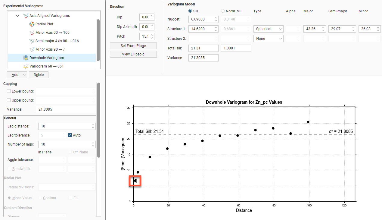
A triangular dragger handle next to the chart’s Y-axis can be used to adjust the Nugget value in the Model Controls part of the window. As the downhole values are nearly continuous, an accurate estimate can be made for the nugget effect for this direction.
Axis Aligned Variograms
The Axis Aligned Variograms are useful for determining the direction of maximum, intermediate and minimum continuity. When you select the Axis Aligned Variograms option, all four variograms are displayed in the chart:
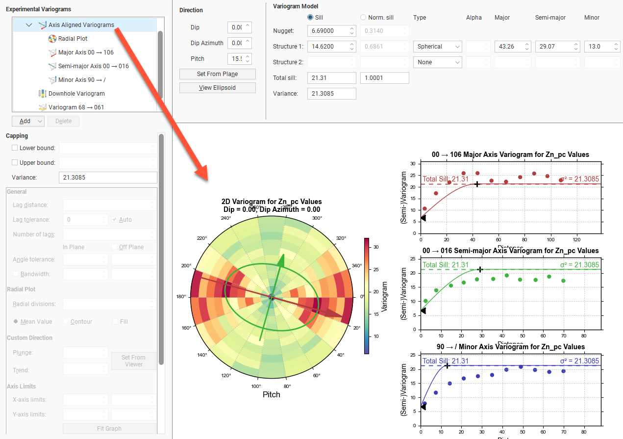
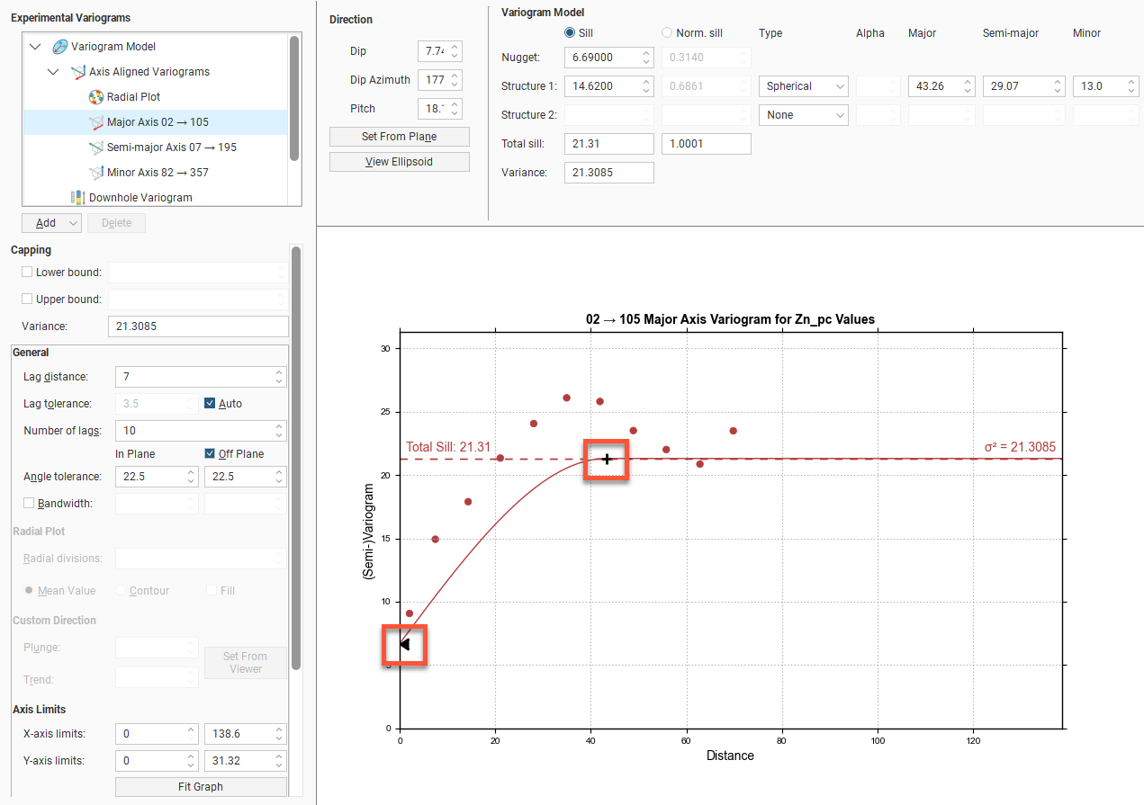
The radial plot and each of the axes variograms can be viewed in greater detail by clicking on them in the variogram tree:
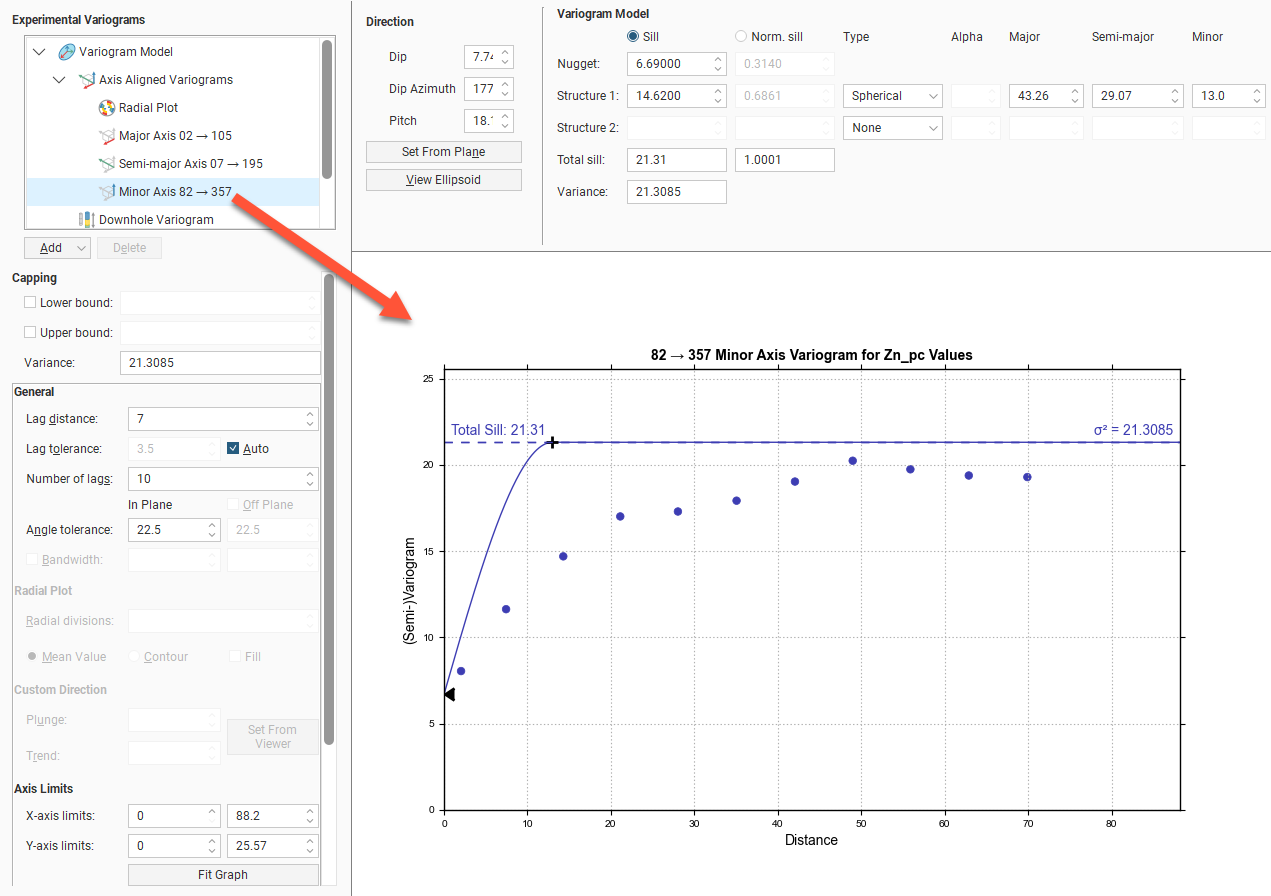
In the axes variogram plots, you can click-and-drag the plus-shaped dragger handle to adjust the range and the sill. A triangular dragger handle adjusts the nugget. A solid line shows the model variogram, and dotted horizontal lines show the Total Sill and, if Sill is chosen instead of Norm. sill, the variance.
Drag handles do not appear on the plots for all display Values options. Handles are not provided for Pairwise Relative because fitting models to pairwise relative variograms is discouraged in the industry. The reason this is discouraged is because the calculation provides a distinctly non-linear re-scaling of the variogram and suppresses the effect of outliers, producing a variogram that is usually optimistic with respect to both nugget and range of continuity.
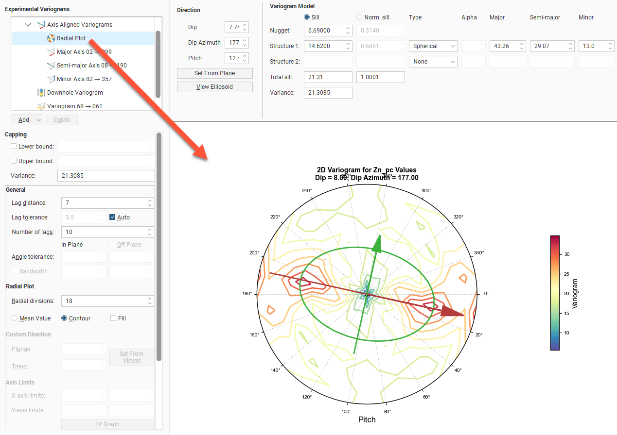
In the radial plot, you can click-and-drag the axes arrows to adjust the pitch setting, between the values 0 and 180 degrees. Each bin in the mean value radial plot shows the mean semi-variogram value for pairs of points binned by direction and distance. When the contour plot is selected, lines follow the points of equal value.
The experimental variogram controls can be different for each axis direction.
Custom Variograms
Any number of custom variograms can be created. These are useful when validating a model, for checking the variogram directions other than the axis-aligned directions. The Plunge to Trend settings determine the direction of the experimental variogram, and these are set independently of the Dip, Dip Azimuth and Pitch settings used by the other experimental variograms. The Plunge to Trend settings can be quickly set by orienting the scene and then clicking the Set From Viewer button in the Variogram Model window. This copies the current scene azimuth and plunge settings into the fields for the custom variogram.
When selected, the custom variogram shows a semi-variogram plot, with the model variogram plotted:
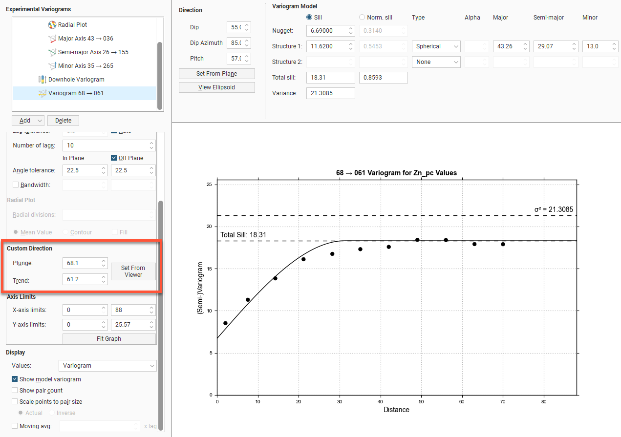
There are no handles on this chart. Dotted horizontal lines indicate the Total Sill and, if Sill is chosen instead of Norm. sill, the variance.