
Variogram Model Controls
The Variogram Model controls adjust the variogram model type, trend and orientation; the graph will update to reflect changes you make to model parameters. The ellipsoid in the scene will also reflect the changes you make to the Variogram Model.
Multi-structured variogram models are supported, with provision for nugget plus two additional structures.
The Nugget represents a local anomaly in values, one that is substantially different from what would be predicted at that point based on the surrounding data. Increasing the value of Nugget effectively places more emphasis on the average values of surrounding samples and less on the actual data point and can be used to reduce noise caused by inaccurately measured samples.
Each additional structure has settings for the component Sill and the normalised sill, labelled Norm. sill, model Type, Alpha (if the model type is spheroidal), and the Major, Semi-Major and Minor ellipsoid ranges.
The Sill defines the upper limit of the model, the distance where there ceases to be any correlation between values. The Sill can be set for the Nugget, Structure 1 and Structure 2.
Piecewise models rise to the Sill at the Range and stay there for increasing distances beyond the Range. Distances beyond the Range in the domain are uncorrelated.
Asymptotic models approach the sill asymptotically near the range and continue to approach it for increasing distances beyond the range. For asymptotic models, the Range parameter used in the model has no equivalent physical meaning, as it does for piecewise models. Common practice is to instead use a scaling of the Range parameter so that the value entered in this screen somewhat mimics the sill/range behaviour of a piecewise model. Typically, this scaling parameter is chosen so that the ‘practical range’ or ‘effective range’ entered corresponds to a point on the asymptotic function that is a defined percentage of the total sill. There is no universally accepted way of defining what this scaling parameter should be. The practical range used in Leapfrog Energy is noted below for each variogram model Type.
A linear model has no sill in the traditional sense, but, along with the ellipsoid ranges, the sill sets the slope of the model. The two parameters Sill and Range are used instead of a single gradient parameter to permit switching between interpolant functions without also manipulating these settings.
The Norm. sill represents the same information as the Sill, but proportionally scaled to a range between 0 and 1, where 1 represents the data Variance. As you select the radio buttons for Sill and Norm. sill, the Y-axis scale on the displayed chart will change to correspond to your selection.
The Total sill is the sum of the component sills for both the data sills and the normalised sills.
The Lock sill icon indicates if the sill is unlocked (![]() ) or locked (
) or locked (![]() ). Click the icon to change the lock state. If unlocked, changing a sill value will adjust the Total sill by the same amount. If locked, adjusting any sill value will not change the Total sill at all, but other sill values will change to keep the Total sill fixed.
). Click the icon to change the lock state. If unlocked, changing a sill value will adjust the Total sill by the same amount. If locked, adjusting any sill value will not change the Total sill at all, but other sill values will change to keep the Total sill fixed.
The Variance is calculated automatically from the data and shows the magnitude of the variance for the data set.
Model Options
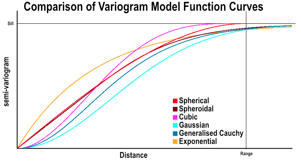
Leapfrog Energy provides a variety of ‘authorised’ variogram model types to ensure the spatial character of continuity can be modelled. ‘Authorised’ variogram models are guaranteed to have the mathematical property of ‘positive definiteness’ for the associated covariance function, meaning the model is guaranteed to produce a valid result when used in Kriging. The model Type provides the options Linear, Spherical, Spheroidal, Gaussian, Exponential, Cubic and Generalised Cauchy.
Variogram models can be bounded or unbounded. Linear is the only unbounded type provided by Leapfrog Energy, where the value of the variogram increases as a linear function of distance. Linear models cannot be combined with the bounded models.
All other model types provided in Leapfrog Energy are bounded models that rise to a sill. These can be separated into two further types:
- Piecewise models that rise to a sill at a range, then are constant beyond that range
- Asymptotic models that approach but never reach a sill
Spherical and Cubic models are piecewise; Spheroidal, Gaussian, Exponential and Generalised Cauchy are asymptotic.
The functions vary in how quickly they rise toward the sill both initially and at (and beyond) the range.
Which function you select will depend on the variable you are modelling, as well as the performance required. For instance, Generalised Cauchy is provided as it is faster than the Gaussian function when applied to an RBF estimator, but provides reasonably similar results.
Variogram model types Cubic, Gaussian and Generalised Cauchy are included specifically for modelling variables with high continuity and local correlation such as dispersed groundwater contaminants. Screening effects and negative Kriging weights can be more pronounced when using these models with continuous behaviour, so use the block model interrogation tool to check the Kriging plan is optimal and the Kriging weights are appropriate.
Each of the variogram model Types are described below. For each, a formula is presented for the model. They all use the following terms:
- γ(h) is the value of the variogram at distance h
- C0 is the sill
- h is the distance on the x axis
- a is the range parameter
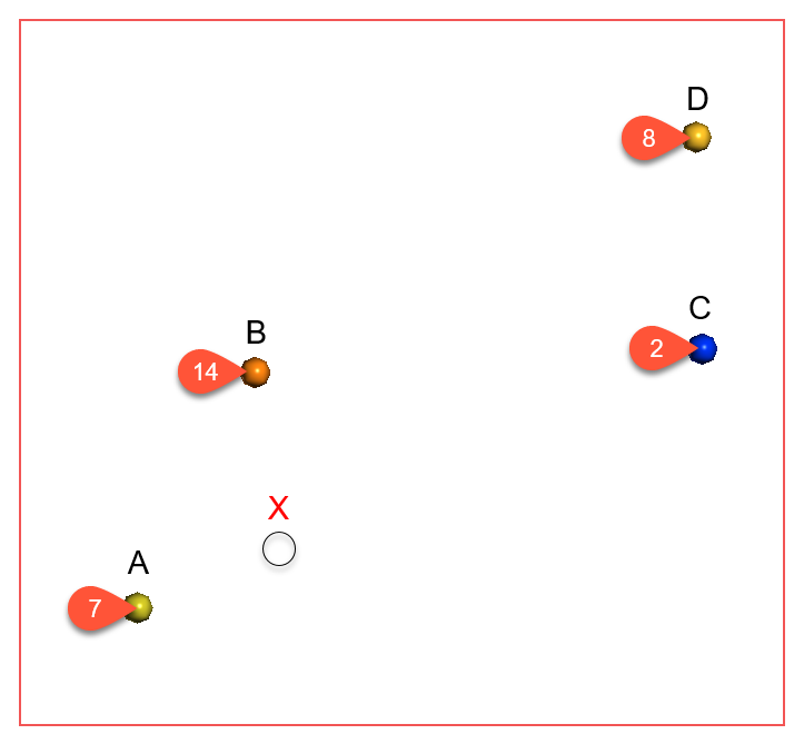
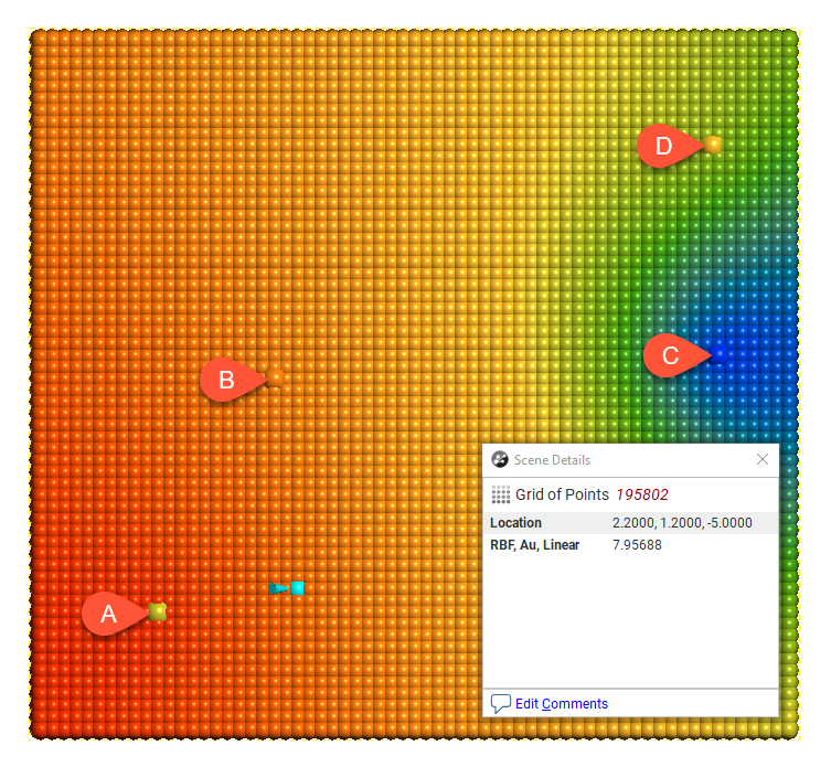
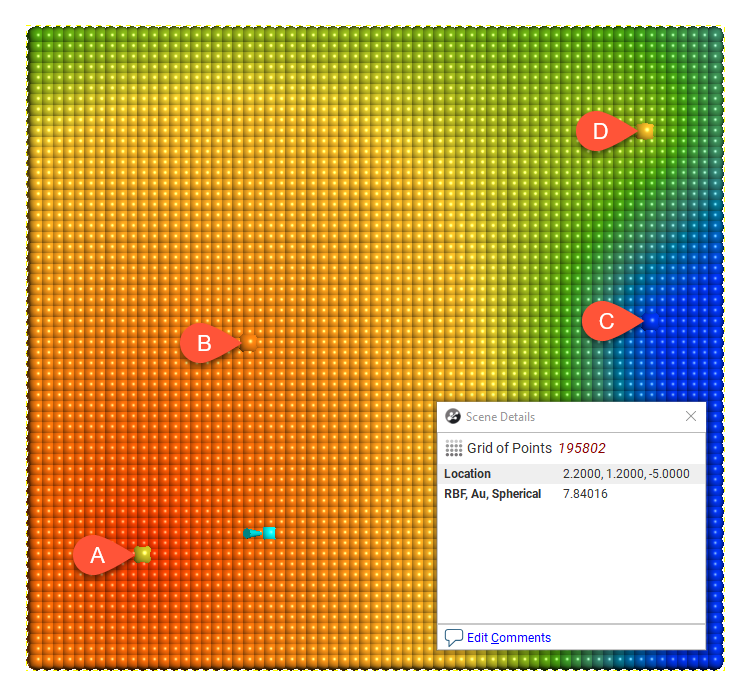
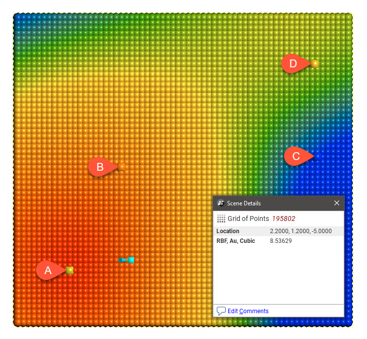
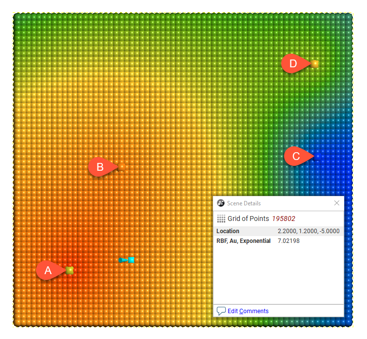
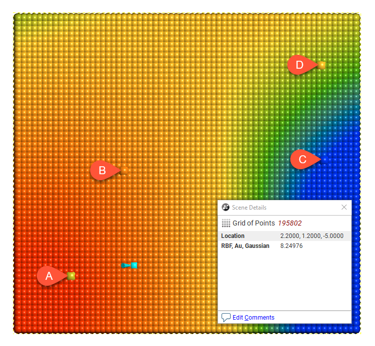
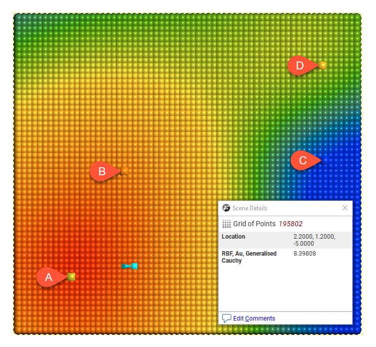
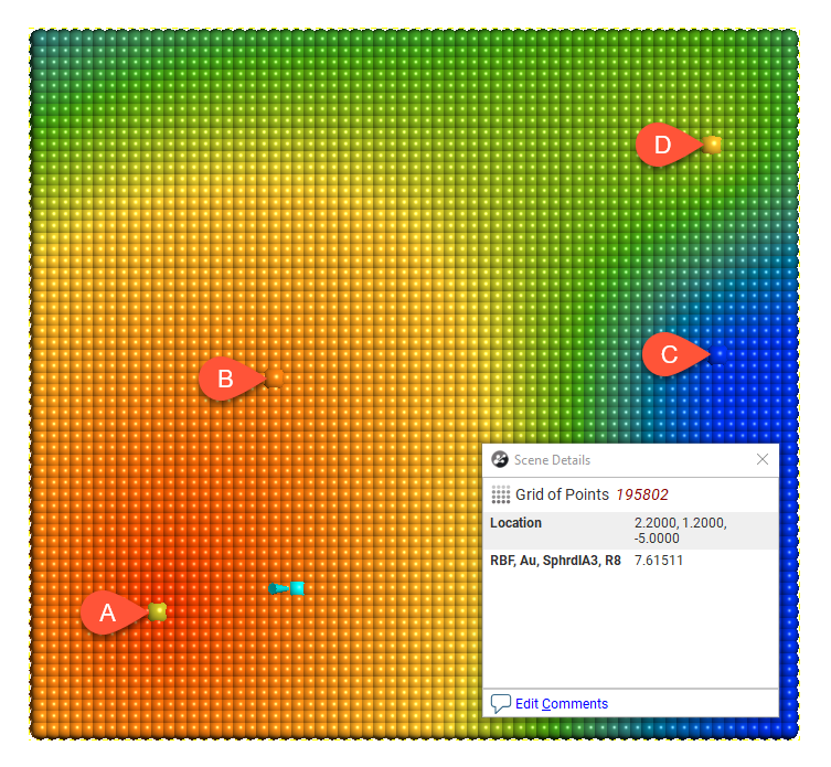
For each model type, the effect of the interpolation function is depicted by evaluation onto a grid of points, using as input just four samples, A = 7, B = 14, C = 2 and D = 8. A thin slice is taken through the grid of points to provide a sort of 2D visualisation of the operation of the function. One of the points has been selected in each view to display the value being estimated for a specific location.
Type = Linear
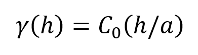
Linear is a general-purpose multi-scale option suited to sparsely and/or irregularly sampled data. It is typically used for modelling of categorical variables.
Type = Spherical
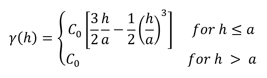
Spherical is suitable for modelling most variables where there is a finite range beyond which the influence of the data should fall to zero. Because the spherical model is piecewise, beyond the range the variogram value is the constant sill.
Type = Cubic
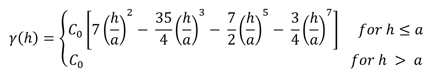
Cubic, like Spherical, is a piecewise model that has a finite range beyond which the influence of the data should fall to zero, and the variogram value is the constant sill. It has been included specifically for modelling variables with high continuity and local correlation such as dispersed groundwater contaminants. Screening effects and negative Kriging weights can be more pronounced when using the cubic model type with continuous behaviour, so use the block model interrogation tool to check the Kriging plan is optimal and the Kriging weights are appropriate.
Type = Exponential
The Exponential variogram model type is used in modelling precious metals such as gold. It has a steeper slope toward the origin than other model types.
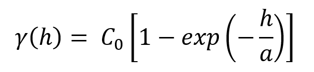
The Exponential model is asymptotic and approaches but never quite reaches the Sill.
An exponential model with a range parameter of a reaches a value of ~95% of the sill at a distance of 3 x a. The Range value is scaled by a factor of 1/3 in the formulation. This has the effect of ensuring that the exponential variogram reaches ~95% of the sill at the ‘practical range’. Beyond the practical range, a point has a small but non-zero correlation.
Type = Gaussian
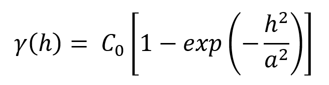
The Gaussian model is asymptotic and approaches but never quite reaches the Sill.
Gaussian has been included specifically for modelling variables with high continuity and local correlation such as dispersed groundwater contaminants. Screening effects and negative Kriging weights can be more pronounced when using these models with continuous behaviour, so use the block model interrogation tool to check the Kriging plan is optimal and the Kriging weights are appropriate.
A Gaussian model with a range parameter of a reaches a value of ~95% of the sill at a distance of √3 x a. The Range value is scaled by a factor of 1/√3 in the formulation. This has the effect of ensuring that the Gaussian variogram reaches ~95% of the sill at the ‘practical range’. Beyond the practical range, a point has a small but non-zero correlation.
Type = Generalised Cauchy
The Generalised Cauchy model is asymptotic and approaches but never quite reaches the Sill.
The Generalised Cauchy covariance can be expressed as:
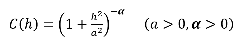
By considering only particular values for the exponent α this expression can be simplified to derive a standardised Generalised Cauchy covariance function of order m, where m = 2α
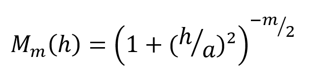
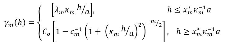
This can in turn be expressed as a variogram function for the Generalised Cauchy variogram of order m:
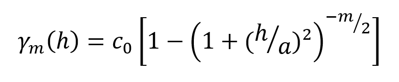
Select the order m by selecting from the Alpha options of 3, 5, 7 or 9, which are the only values allowed in Leapfrog Energy. For a given range parameter a, the variograms of order m reach the same proportion of total sill at quite difference distances. In order to equate the shape of the variogram to the entered Range parameter, scaling parameters are applied.
For a Generalised Cauchy variogram of order 9, the value of γ at the specified range parameter is 95.58% of the total sill. Because the convention is arbitrary, Leapfrog Energy considers that a variogram of order 9 does not require a re-scaling of the range parameter. Leapfrog Energy then uses this sill proportion of 95.58% to calculate scaling factors for variograms of order 3, 5 and 7. In practice, a lookup table is used with ideal values rounded to 10 decimal places:
| Order (m) | Range scaling factor |
| 3 | 0.3779644730 |
| 5 | 0.6347188807 |
| 7 | 0.8339047224 |
| 9 | 1.0000000000 |
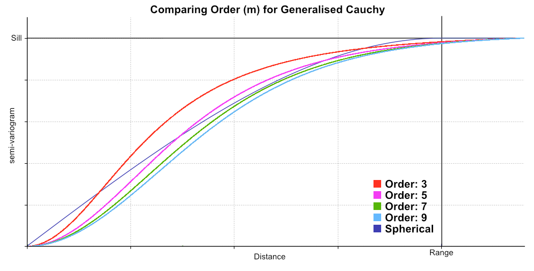
This has the effect of ensuring that the Generalised Cauchy variogram reaches 95.58% of the sill at the ‘practical range’. Beyond the practical range, a point has a small but non-zero correlation. For further details on the derivation see The Spheroidal Family of Variograms Explained on the Seequent blog.
This chart shows the relative differences for different values of Alpha, which is the order (m) of the function, in comparison to a spherical curve:
Type = Spheroidal
The Spheroidal model is asymptotic and approaches but never quite reaches the Sill. However, the first part of the function is linear.
Spheroidal is suitable for modelling most variables where there is a finite range beyond which the influence of the data should fall to zero. The spheroidal variogram was developed by Seequent primarily for use in RBF interpolants. Seequent wanted an effectively compact spatial function that has linear behaviour near the origin and an asymptotic approach to the sill. This was developed by taking a commonly used family of radial functions and linearising them near the origin. This results in a variogram that combines the Linear model with the Generalised Cauchy variogram model. The transition point between these two is the inflection point on the Generalised Cauchy model.
where
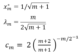
Select the order m by selecting from the Alpha options of 3, 5, 7 or 9, which are the only values allowed in Leapfrog Energy. For a given range parameter a, the variograms of order m reach the same proportion of total sill at quite difference distances. In order to equate the shape of the variogram to the entered Range parameter, scaling parameters are applied.
For a Spheroidal variogram of order 9, the value of γ at the specified range parameter is 96% of the total sill with no nugget. Because the convention is arbitrary, Leapfrog Energy considers that a variogram of order 9 does not require a re-scaling of the range parameter. Leapfrog Energy then uses this sill proportion of 96% to calculate scaling factors for variograms of order 3, 5 and 7. In practice, a lookup table is used with ideal values rounded to 10 decimal places:
| Order (m) | Range scaling factor |
| 3 | 0.3731574337 |
| 5 | 0.6319995630 |
| 7 | 0.8327312240 |
| 9 | 1.0000000000 |
This has the effect of ensuring that the Spheroidal variogram reaches 96% of the sill at the ‘practical range’ with no nugget. Beyond the practical range, a point has a small but non-zero correlation. For further details on the derivation see The Spheroidal Family of Variograms Explained on the Seequent blog.
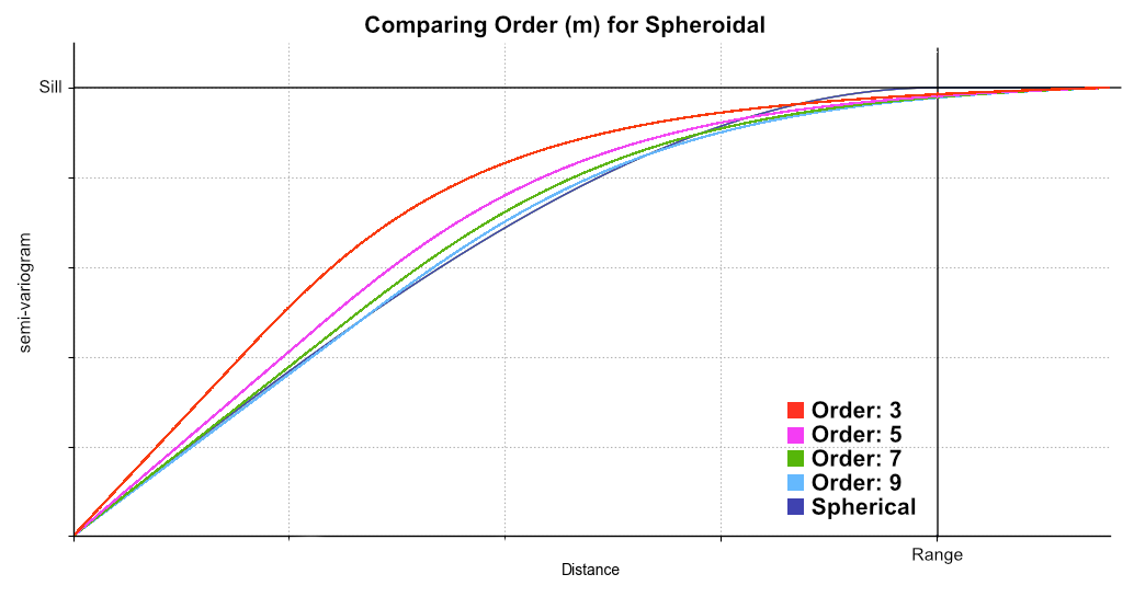
This chart shows the relative differences for different values of Alpha, which is the order (m) of the function, in comparison to a spherical curve:
The spherical model is not available for standard Leapfrog RBF interpolants created in the Numeric Models folder.
Alpha is only available when the model Type is Spheroidal or Generalised Cauchy. The Alpha constant determines how steeply the interpolant rises towards the Sill. A low Alpha value will produce a variogram that rises more steeply than a high Alpha value. A high Alpha value gives points at intermediate distances more weighting, compared to lower Alpha values. An Alpha of 9 provides the curve that is closest in shape to a spherical variogram. In ideal situations, it would probably be the first choice; however, high Alpha values require more computation and processing time, as more complex approximation calculations are required. A smaller value for Alpha will result in shorter times to evaluate the variogram.
RBF estimators will only work when the Structure 2 model Type is set to None.
When Structure 2 is defined, the model ranges cannot be adjusted by manipulation of drag handles on the ellipsoid. Because it would not be clear which structure was being manipulated, the drag handles to change the range settings do not appear.
Normalised Y Axis
A key use of copying a variogram is to apply it to another correlated contaminant. This would typically be accomplished, having determined the appropriate variogram using the values for one contaminant, by copying the domained estimation and changing the Numeric values field to a different contaminant. However, the absolute values for the nugget and sills for each structure would be completely inappropriate for the new contaminant; while we desire the shape to be the same, the values for different compounds will inevitably be different. To make this work correctly, the variogram is normalised or standardised, rescaling the range of Y-axis values to between 0 and 1, where 1 is equivalent to the data Variance. This makes the variogram information portable between domained estimations. This is performed automatically, requiring no intervention on your part.
You can freely switch between the Sill and Norm. sill options. The selection only changes the Y-axis scale on the displayed chart.
You do not need to select the Normalised option before copying the domained estimation and using it as the basis for a different mineral resource. The normalised scale will always be used when applying the variogram model to the new data set.
As you adjust the Nugget or the Structure 1 or Structure 2 sill values, the Total sill will change both for the absolute Sill values and the Norm. sill values. The Norm. sill total may end up being something other than 1.0. This is expected, as the value reference for the normalised scale uses the data Variance for 1.0, not the total sill.
Note that the data Variance is recorded in the Y axis label so the chart scale is always meaningful, including when the chart is exported.
Direction
The trend Direction fields set the orientation of the variogram ellipsoid. Adjust the ellipsoid axes orientation using the Dip, Dip Azimuth and Pitch fields.
The Set From Plane button sets the trend orientation of the model ellipsoid based upon the current settings of the moving plane.
The View Ellipsoid button adds a 3D ellipsoid widget visualisation to the scene, in case it has been deleted from the scene since the variogram model window was opened for editing.