Trends and Anisotropy

A point source of light radiates in all directions equally, and the intensity of that radiated light decreases at a rate equal to the inverse of the square of the distance from the source. This radiation is isotropic, and in many fields isotropic behaviour can be assumed when making measurements. Geologists are well aware that, in their field, this cannot be assumed. Because of the processes involved in rock and strata formation involving sedimentation, compression and igneous flows, measurements can demonstrate strong trends in one particular direction or plane, but weak trends in an orthogonal direction.

Structural data is used to inform analysis of directional behaviour, for visualisation and/or modelling of trends. Leapfrog Energy uses the following structural data types:

• Planar structural data disks
• Lineations
• Triaxial ellipsoids

For more on these input data types, see the Structural Data topic.

The Ellipsoid Widget

To communicate trends and anisotropy in the scene, Leapfrog Energy uses the ellipsoid widget:

• To visualise anisotropy proportions and orientation
• To visualise the variogram model in the scene, including rotation and ranges
• To depict search neighbourhoods

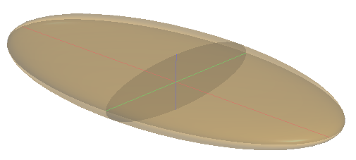
To assist in visualising the orientation and shape of the ellipsoid, in most instances ellipsoid widgets will have axes lines and translucent internal planes. The major, semi-major and minor axes are also drawn as red, green and blue lines respectively. Translucent planes will be seen within the ellipsoid if the opacity of the ellipsoid is reduced.

Usually, the planes show the major/semi-major plane and the semi-major/minor plane.

Ellipsoid widgets can be repositioned, perhaps so the ellipsoid is not obstructing the view of part of the model. To reposition the widget, select the widget in the shape list then click on the widget in the scene. If the ellipsoid does not have arrows in its centre, click the ellipsoid; the movement arrows will appear. You can click the ellipsoid again to turn the movement handles off.

In the properties panel for the selected widget, settings control the Centre Point of the ellipsoid. The X, Y and Z position can be specified directly.

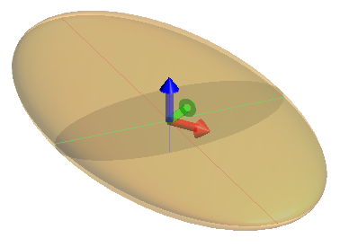
There are two modes for the widget movement handles. In the properties panel for the selected widget, Align movement handles to has the options Axes and Camera.

When set to Axes, the drag handles in the centre of the widget will be red, green and blue and point along the directions of the project axis lines. You can click on one of the red, green or blue movement handles and drag it in the scene, and the ellipsoid will move forward or back in the direction of the selected project axis.

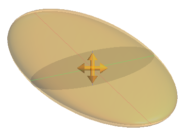
When set to Camera, the drag handles in the centre of the widget will be orange and point up/down/left/right across the scene view. You can click anywhere on the orange handles and drag the widget in the scene; the ellipsoid will move across the viewing plane.

Where ellipsoid widgets are used to depict a structural trend, ellipsoid axes and planes are not shown, and movement handles are not available.

Modelling Trends

Leapfrog Energy provides tools to account for anisotropy when modelling, including:

• Global Trends
• Structural Trends
• Variable Orientations
• Variography

To visually convey the magnitude and directionality of a trend, Leapfrog Energy uses a visual element called the ellipsoid widget. For more, see The Ellipsoid Widget above.

Understanding Anisotropic/Ellipsoidal Distance

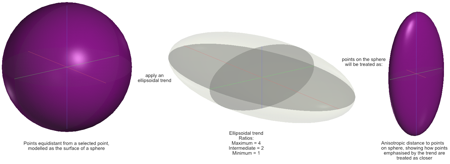
When a trend is applied during modelling, distances between points are scaled proportionally to the ellipsoidal trend, creating a concept called the anisotropic distance, or ellipsoidal distance. When interpolating to calculate a value at a specific point, measured data points closer to that point will have more influence in the interpolation calculation. When a trend is applied, the anisotropic distance is used instead of the actual distance. In the trend’s maximum direction we want the measured data points to have more influence, so the anisotropic distance is smaller than the actual distance. We divide the actual distance by the maximum axis ratio, so if the ellipsoid maximum ratio is 4, the anisotropic distance to a point in the maximum direction is ¼ the actual distance, significantly increasing the influence of a measured point in that direction. If the intermediate ratio is 2, the anisotropic distance to a point in the intermediate direction is ½ the actual distance, again increasing the influence of a measured point in that direction, though not as significantly as in the maximum direction. Consider this diagram demonstrating how points equidistant from a central point are treated when an anisotropic trend is applied, with the ratios maximum = 4, intermediate = 2 and minimum = 1.

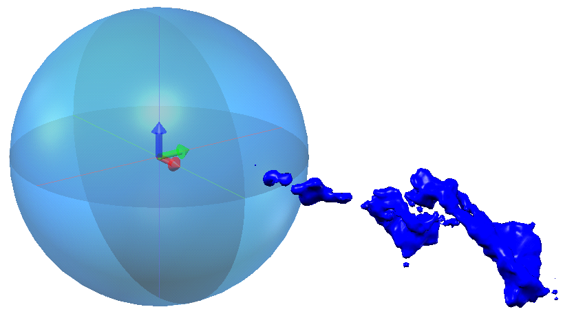
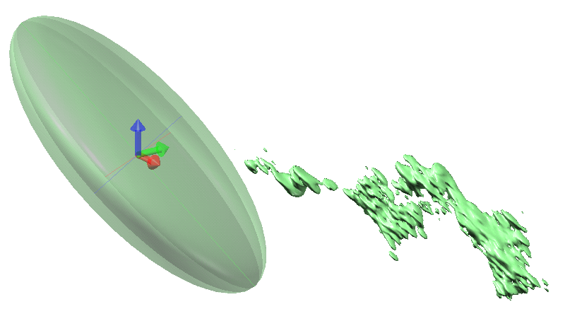
It may be useful to think of the ellipsoidal trend as warping spacetime, making the apparent anisotropic distance or ellipsoidal distance shorter in emphasised directions. Still, it is not normally necessary to envisage things by anisotropic distances. More intuitively, interpolated surfaces modelled using trends clearly demonstrate the emphasis indicated by the trend ellipsoid proportions and orientation.

When it’s necessary to make it clear that we are talking about an actual isotropic or cartesian distance between two points independent of any anisotropic trend, Leapfrog Energy uses the term Euclidean distance.

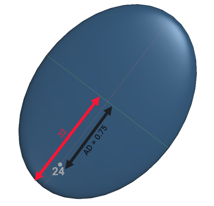
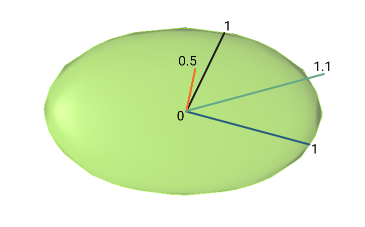
Anisotropic distances are not stored in project units, as this would create additional confusion. Instead, anisotropic distances such as MinAD and AvgAD are stored as proportions of a reference surface. In the case of MinAD and AvgAD, it is the search ellipsoid. All points lying on the surface of the ellipsoid have a value of 1 relative to the centre of the search ellipsoid. Consider a point within the search ellipsoid: A line drawn from the centre of the ellipsoid through that point to the surface of the ellipsoid extends from the 0 distance at the centre to the surface at anisotropic distance 1. The anisotropic distance of the point from the centre will be between 0 and 1, in proportion to its position along that line. If a point is outside the surface, the anisotropic distance would be greater than 1.

If a point happens to lie on one of the orthogonal axes for the anisotropic trend, it is simple to convert from anisotropic distance to Euclidean distance. The Euclidean distance = anisotropic distance * ellipsoid range for that axis. For instance, if a point lies on the maximum axis for the search ellipsoid with a range of 32, and the anisotropic distance is 0.75, then the Euclidean distance is 24. The calculation for any point not along the axes requires only a little more basic trigonometry to solve.