
Numeric Composites
Compositing numeric data takes unevenly-spaced drilling data and turns it into regularly-spaced data, which is then interpolated. Compositing parameters can be applied to entire wells or only within a selected region of the well. For example, you may wish to composite Au values only within a specific lithology.
There are two approaches to compositing numeric data in Leapfrog Energy:
- Composite the drilling data directly. Compositing parameters can be applied to entire wells or only within a selected region of the well. This creates a new interval table that can be used to build models, and changes made to the table will be reflected in all models based on that table. This process is described below.
- Composites the points used to create an interpolant. This is carried out by generating an interpolant and then setting compositing parameters for the interpolant’s values object. This isolates the effects of the compositing as the compositing settings are only applied to the interpolant.
Intervals that have no data can have a significant effect when compositing data as they are ignored by the compositing algorithm. The effect of these missing intervals can be managed using the Minimum coverage parameter, but it’s best to assign special values where intervals have no data. For example, intervals that are missing data can be assigned a value of 0 or that of the background mineralisation. See Handling Special Values for more information.
The rest of this topic describes compositing drilling data directly. It is divided into:
- Creating a Numeric Composite
- Compositing in the Entire Well
- Compositing in a Subset of Codes
- Using Intervals From Another Table
- Using Intervals with Advanced Upscaling
- Viewing Numeric Composite Statistics
Creating a Numeric Composite
Creating a numeric composite involves the following steps:
- Selecting the compositing region
- Setting the composite length
- Setting residual length handling
- Setting coverage
- Selecting an additional weighting column (optional)
- Selecting the output columns
To start the process of creating a numeric composite, right-click on the Composites folder and select New Numeric Composite. You will be prompted to select the compositing region.
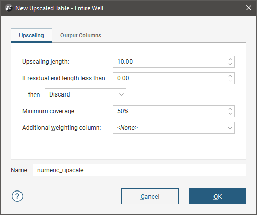
- Entire Well. The same compositing parameters are applied to all values down the length of wells, regardless of unit breaks. See Compositing in the Entire Well.
- Subset of Codes. Different compositing parameters can be set for each code down the length of wells. See Compositing in a Subset of Codes.
- Intervals from other Table. Interval lengths from another table are used to determine composite lengths. The value assigned to each interval is the length-weighted average value, and there are no further compositing parameters to set. See Using Intervals From Another Table.
- Intervals from other Table with Advanced Upscaling. Interval lengths from another table are used to determine upscale lengths and advanced upscaling algorithms are set. See Using Intervals with Advanced Upscaling.
Each option requires a different set of compositing parameters, which are described below.
Once you have set up the composite, click OK to create the table, which will be saved to the Composites folder. Double-clicking on the table displays the data in its columns. Edit the table by right-clicking on it and selecting Edit Composited Table. You can view statistics on the table or for each individual column in the table. See Viewing Numeric Composite Statistics.
Compositing in the Entire Well
When compositing is carried out using the Entire Well option, the wells are divided into intervals wherever numeric data occurs and the parameters set in the Compositing tab are applied to all values down the length of wells.
The order of the operations in numeric compositing is as follows:
- A compositing length is selected. This may or may not end up being the exact length of composited intervals, which will depend on subsequent parameters and the actual data.
- Determine how to handle short sections at the end of wells that are shorter than the compositing length.
- If Distribute equally throughout well is selected, all the composited intervals will grow longer than the compositing length.
- If Add to previous interval is selected, the last interval will be longer than the compositing length.
- Compare the total length of data in each composited interval to the Minimum coverage parameter. If the available data does not meet the threshold for an interval, that interval will not get a composited value.
- Determine how to weight the input data, if required.
- Derive a value for each of the composited intervals that passes the minimum coverage test.
Compositing Length
The Compositing length you set will depend on factors including the deposit style, the sampling method and raw sample length. You can view statistics on the drilling data table to get an idea of the distribution of interval lengths. Right-click on the drilling data table and select Statistics. In the window that appears, select the Interval Length Statistics option:
Another consideration in selecting the composite length is choosing a length that will not split units. For example, if most intervals are 2m long, choosing a length of 1m or 5m will split some intervals so that an interval with a single value will be represented more than once in the composite intervals. If intervals are mostly 2.5m long, then a composite length that is 2.5m or a multiple of 2.5m would ensure that units are not split.
Note that the actual length of intervals in the composited table may be longer than that set by the Compositing length. This arises from residual segments at the ends of wells and where there is data missing down a well; the length of these residual segments will, in certain conditions, be added to the composite intervals further up the well. See Residual End Length Handling below for more information.
Residual End Length Handling
The full length of each well will seldom divide up exactly into a whole number of intervals of the specified Compositing length. For this reason, “residual segments” will occur at the end of each well and where there is data missing down the length of the well. In the Compositing tab, you can set a residual end length value, which is the threshold at which all short residual segments will simply be treated as composited intervals. You can then specify how residual segments that are shorter than the residual end length are handled. Options are:
- Discard. If the residual segment is shorter than the Residual end length for a composited interval, it is discarded.
- Add to previous interval. If the residual segment is shorter than the Residual end length for a composited interval, it is added to the previous interval. Note that when this occurs, the actual length of that last composited interval will be longer than the Compositing length specified.
- Distribute equally throughout well. If the residual segment is shorter than the Residual end length for a composited interval, the extra length is divided up and distributed to each of the other intervals. Note that when this occurs, the actual length of each composited interval will be longer than the Compositing length specified.
When the residual segment is longer than the residual end length but the length of provided data within the residual segment also meets or exceeds the Minimum coverage for a composited interval, the residual segment will simply be treated as a composited interval, although it is shorter than the typical intervals. When the Minimum coverage proportion is not achieved, the data is discarded. See Minimum Coverage below for more information on this setting.
In the illustration below, a series of adjacent wells have varying lengths of small data intervals that will not make up a full composited interval. The Residual end length is 5, the option to Distribute equally throughout well has been selected and the Minimum coverage is 32%. The well data is shown in the centre, with the composited data shown around the wells.
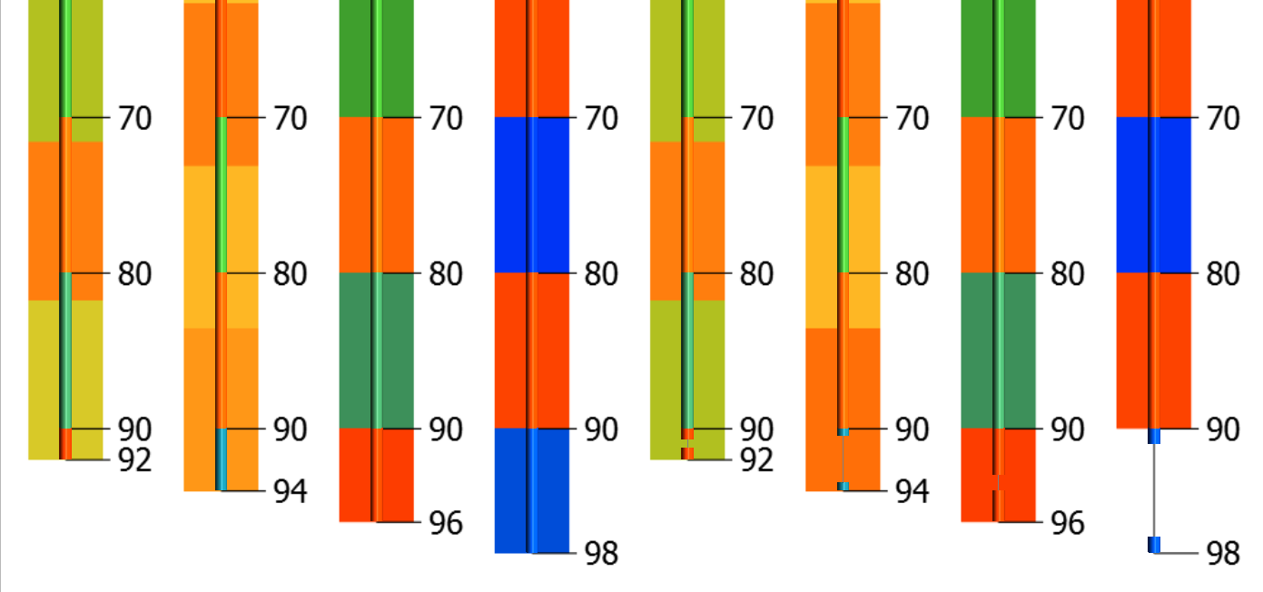
The left four wells have extra residual segments of 2m, 4m, 6m and 8m. The two wells with short lengths less than 5m show the extra length has been distributed across the well intervals for compositing, as seen by the well interval transitions not lining up with the 10m depth markers. The wells with extra lengths of 6m and 8m have had the lengths added as short composite intervals, as they exceeded the residual end length.
The right four wells have missing data of varying lengths. Again, the two wells on the left have had the residual segment length distributed across the well intervals for compositing, as seen by the interval transitions not lining up with the 10m depth markers. Even though the 4m residual end segment has only 25% data coverage, the selected action is applied because the residual segment is shorter than the residual end length. The 6m residual end segment has 83% data coverage, so the additional segment is added as a short composited interval. The 8m residual end segment on the very right has only 25% data coverage, so the data is discarded.
Minimum Coverage
The Minimum coverage parameter determines whether or not a value will be calculated for a composite interval, based on the data available in the input data table. The Minimum coverage is a threshold the input intervals must meet in order for a composited value to be calculated. If, for example, the Minimum coverage is 50%, a value will be calculated for a composite interval only when there is data in at least 50% of the well that informs the composited interval.
- Setting Minimum coverage to 100% will result in composite intervals being assigned values only when there is data for all well intervals that inform the composite interval.
- Setting Minimum coverage to 0% will result in all composite intervals being assigned values, even where input intervals have no data.
In the image below, several adjacent wells have various sized gaps in the drilling data, shown using the inner solid line. The outer translucent line represents the composited intervals, and as the Minimum coverage value was set at 32%, only the largest data gap resulted in a missing composited interval.
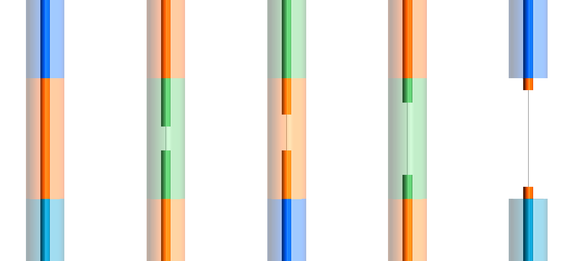
Intervals that have no data can have a significant effect when compositing data as they are ignored by the compositing algorithm. The effect of these missing intervals can be managed using the Minimum coverage parameter, but it’s best to assign special values where intervals have no data. For example, intervals that are missing data can be assigned a value of 0 or that of the background mineralisation. See Handling Special Values for more information.
Composite values are calculated for each composite interval. This is simply the length-weighted average of all numeric drilling data that falls within the composite interval.
Composite points are generated at the centre of each composite interval from the composite values.
Additional Weighting Column
If you use an Additional weighting column, the column selected must contain valid (positive) values for all of the composite’s output intervals. If this is not the case, you will receive a message saying the table cannot be created. If the column selected as the weighting column is also in the list of output columns, that output column will be composited using length-weighted averaging only.
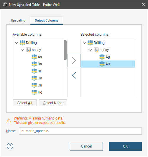
Output Columns
In the Output Columns tab, select the columns to be added to the numeric composite table. Move selected items from the Available columns list to the Selected columns list by clicking an item then clicking the ![]() button. You can select multiple items by holding down Ctrl while clicking.
button. You can select multiple items by holding down Ctrl while clicking.
Search for items in a list by pressing Ctrl-F. A Find window will appear that you can use to search the list. You can choose whether or not to match case in the search and whether or not to match the whole label. You can search forwards or backwards and you can select all list items that match the current search.
Compositing in a Subset of Codes
When compositing is carried out using the Subset of Codes option, some codes can be excluded from the composited table or the raw data from the Base column can be used. When compositing is applied to a code, the same parameters apply as for the Entire Well option, but different codes can use different Compositing length and Minimum coverage parameters.
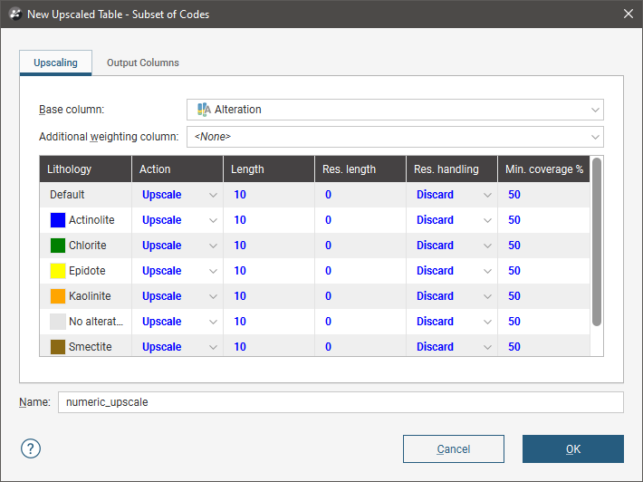
For the Action column, select from:
- Composite. Numeric data that falls within the selected code will be composited according to the parameters set.
- No compositing. Numeric data is not composited within the selected code. The raw data will be used in creating the new data table.
- Filter out. Numeric data within the selected code will excluded from the new data table.
See Compositing in the Entire Well above for an explanation of the Length, Min. coverage, Res. length, Res. handling and Additional weighting column parameters.
Once you have set the compositing parameters, click on the Output Columns tab to select from the available columns of numeric data. See Output Columns above for more detail.
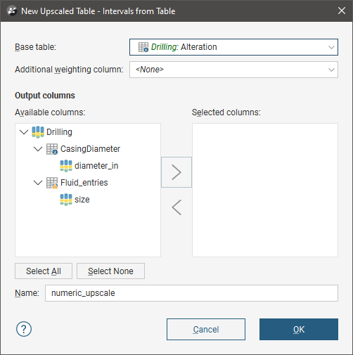
Using Intervals From Another Table
When compositing is carried out using the Intervals from other Table option, first select the Base table. This is the table that will that will be used to determine the interval lengths in the composited table.
Search for items in a list by pressing Ctrl-F. A Find window will appear that you can use to search the list. You can choose whether or not to match case in the search and whether or not to match the whole label. You can search forwards or backwards and you can select all list items that match the current search.
The value assigned to each interval will be the length-weighted average value, and you can use an Additional weighting column. This column must contain valid (positive) values for all of the composite’s output intervals. If this is not the case, you will receive a message saying the table cannot be created. If the column selected as the weighting column is also in the list of output columns, that output column will be composited using length-weighted averaging only.
There are no further compositing parameters to set. Click OK to create the table.
Using Intervals with Advanced Upscaling
When compositing is carried out using the Intervals from other Table with Advanced Upscaling option, first select the Base table and the Sampling method. You can also select an Additional weighting column, but note that this will only apply when the Arithmetic algorithm is selected.
There are two options for Sampling method:
- Whole interval. All data points in the upscaled interval are taken into account when calculating the upscaled value for that interval.
- Dominant category. A Category column is selected that determines whether or not data points in the upscaled interval are taken into account. Data points in the interval that do not occur in the dominant category are not used in calculating the upscaled value for that interval.
Then select which Output columns you wish to include. You can then set the Algorithm and 0 replacement value for each column:
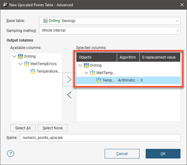
Available algorithms are Arithmetic, Geometric, Harmonic, Max, Median and Min.
Click OK to create the table.
Viewing Numeric Composite Statistics
Once you have created a composited table, you can view statistics on the table or for each individual column in the table.
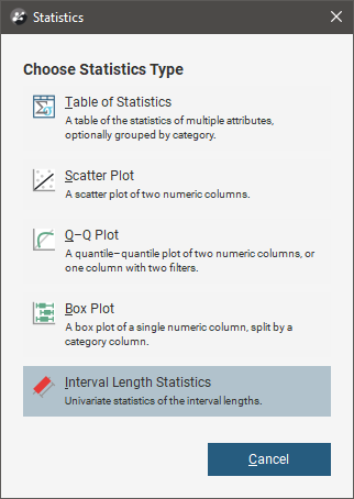
To view statistics for the table, right-click on it and select Statistics.
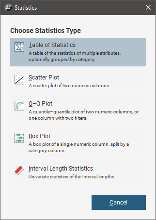
See the Statistics topic for more information on each option:
The Interval Length Statistics graph is a univariate graph, so for more information on the options available, see Univariate Graphs in the Statistics topic.
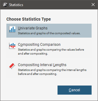
Right-click on the table columns and select Statistics to view information about the composited values.
The first option displays statistics on the composited values. The other two options display statistics comparing data before and after compositing.
Compositing Comparison
Declustering Comparison charts are similar to Compositing Comparison charts but have the addition of Input Values. See Comparison Histograms for more detail.
The double histogram, one displaying the distribution of the raw data and one displaying the distribution of the composited data, enables comparison of the two distributions of the same element before and after the compositing transformation. Impacts on the symmetry of distributions will be evident.
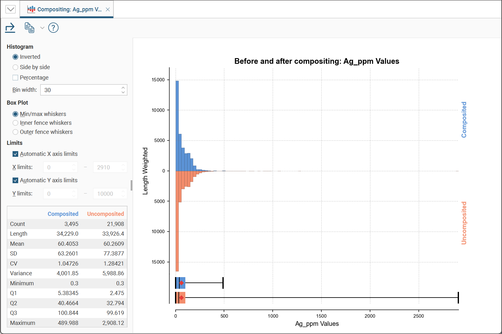
In the Histogram settings, you can choose between Inverted graphs, as shown in the image above, or Side by side graphs where the data for each histogram bin is shown in the traditional histogram style. Bin width changes the size of the histogram bins used in the plot.Percentage is used to change the Y-axis scale from a length-weighted scale to a percentage scale.
The Box Plot options control the appearance of the box plot drawn under the primary chart. The whiskers extend out to lines that mark the extents you select, which can be the Min/max whiskers, the Inner fence whiskers or the Outer fence whiskers. Inner and outer values are defined as being 1.5 times the interquartile range and 3 times the interquartile range respectively.
The Limits fields control the ranges for the X-axis and Y-axis. Select Automatic X axis limits and/or Automatic Y axis limits to get the full range required for the chart display. Untick these and manually adjust the X limits and/or Y limits to constrain the chart to a particular region of interest. This can effectively be used to zoom the chart.
The bottom left corner of the chart displays a table with a comprehensive set of statistical measures for the dataset.
Compositing Interval Lengths
This graph shows a double histogram of distributions of the interval lengths before and after compositing.
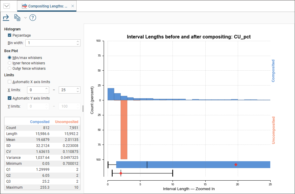
In the Histogram settings, Bin width changes the size of the histogram bins used in the plot.Percentage is used to change the Y-axis scale from a length-weighted scale to a percentage scale.
The Box Plot options control the appearance of the box plot drawn under the primary chart. The whiskers extend out to lines that mark the extents you select, which can be the Min/max whiskers, the Inner fence whiskers or the Outer fence whiskers. Inner and outer values are defined as being 1.5 times the interquartile range and 3 times the interquartile range respectively.
The Limits fields control the ranges for the X-axis and Y-axis. Select Automatic X axis limits and/or Automatic Y axis limits to get the full range required for the chart display. Untick these and manually adjust the X limits and/or Y limits to constrain the chart to a particular region of interest. This can effectively be used to zoom the chart.
The bottom left corner of the chart displays a table with a comprehensive set of statistical measures for the dataset.