
GM-SYS 3D Models
A GM-SYS 3D model describes a volume of earth, extending from a top surface (usually topography or sea level) to a specified bottom elevation. The horizontal extents of a model are defined by selecting an index grid or voxel, from which the horizontal cell size, number of samples, projected coordinate system, and horizontal units of the model are copied. The model volume may then be divided into sub-volumes of differing physical properties to build a more realistic representation of the density within the Earth. Layer tops may be partially or completely coincident, causing a layer to be zero thickness where coincident, but they may never cross.
Each layer or body in a model may be assigned different values for each supported physical property (density, susceptibility, remanent magnetization, and velocity) in order to build a realistic 3D representation of the property distributions within the Earth. Layer density may be specified using either a constant density, a vertical density gradient, a laterally-varying density distribution, or a distribution that varies in three dimensions. Layer susceptibility may be specified using either a constant susceptibility and remanent magnetization, a laterally-varying susceptibility distribution or a distribution that varies in three dimensions. Layer velocity may be a constant.
In order to calculate the response of the model, you must add a gravity and/or magnetic survey defining how and where the response should be calculated. A survey defines the location of the calculations, appropriate background field information, and optionally may include observed data components and inline filtering parameters.
3D Model Example
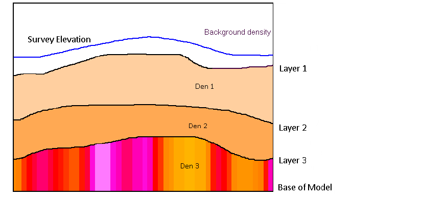
The image below illustrates a three-layer gravity model. Each layer is defined by a top relief surface and a density distribution for the volume below the relief surface.
Got a question? Visit the Seequent forums or Seequent support
© 2023 Seequent, The Bentley Subsurface Company
Privacy | Terms of Use