Geophysical Data

The types of geophysical data that can be imported into Leapfrog Geo are:

• 2D Grids
• 2D and 2D Crooked SEG-Y Data (with Geophysics extension)
• 3D SEG-Y Data (with Geophysics extension)
• ASEG_DFN Files
• UBC Grids
• GOCAD Models
• Magnetotelluric Resistivity Files (with Geophysics extension)

2D Grids

Leapfrog Geo imports the following 2D grid formats:

• Arc/Info ASCII Grid (*.asc, *.txt)
• Arco/Info Binary Grid (*.adf)
• Digital Elevation Model (*.dem)
• ESRI .hdr Labelled Image (*.img, *.bil)
• Geosoft Grid (*.grd)
• Grid eXchange File (*.gxf)
• Intergraph ERDAS ER Mapper 2D Grid (*.ers)
• SRTM .hgt (*.hgt)
• Surfer ASCII or Binary Grid (*.grd)

To import a 2D grid, right-click on either the Geophysical Data folder and select Import 2D Grid. Navigate to the folder that contains grid and select the file. Click Open to begin importing the data.

The Import 2D Grid window will appear, displaying the grid and each of the bands available. Select the data type for each band and set the georeference information, if necessary. See Importing a Map or Image for information on georeferencing imported files.

Once the grid has been imported, you can set its elevation, which is described in Setting Elevation for GIS Objects and Images.

When you display the grid in the scene, select the imported bands from the shape list:

Grids can be displayed as points () or as cells and the values filtered, as described in Displaying Points.

2D and 2D Crooked SEG-Y Data

Leapfrog Geo imports 2D and 2D crooked SEG-Y data in *.segy and *.sgy formats. External navigation files are not supported.

To import 2D SEG-Y data, right-click on the Geophysical Data folder and select Import 2D SEG-Y. Leapfrog Geo will ask you to specify the file location. Click Open to start importing the file.

Leapfrog Geo will read the data in the file and match the data to the expected format. In most cases, Leapfrog Geo will set the correct values from the information in the file.

There are two steps to work through. First, set up the Key Field Locations. There are buttons at the top of the window for displaying the Text Header and Binary Header, which may be useful in deciding what import settings to use.

Settings for setting the Key Field Locations are:

• Byte order. This will be Big endian or Little endian and must be correct in order for the other data in the file to be read correctly.
• Samples per trace. This is the number of samples in each trace. If the correct value cannot be read from the file, you can set it manually by selecting User from the Source dropdown list.
• Sample interval. This is the vertical sample spacing for the trace data and is almost always stored in thousandths of true units. If the correct value cannot be read from the file, you can set it manually by selecting User from the Source dropdown list.
• First sample at. This is the delay recording time for the first sample. If the correct value cannot be read from the file, you can set it manually by selecting User from the Source dropdown list.
• Last sample location. This is read-only and is the calculated location from the last sample in the trace.
• Trace data format. This should be defined in the binary header.

Click Next to move on to setting the Coordinate Field Locations. In this step, the More button displays the trace header fields:

Settings for setting the Coordinate Field Locations are:

• Inline. This is the location in the trace header of the in-line coordinate.
• Crossline. This is the location of the cross-line location.
• X. This is the location of the X-coordinate of the trace location.
• Y. This is the location of the Y-coordinate of the trace location.
• Scalar. This the coordinate scale factor used for ground coordinates. It is read-only, but you can choose to disable the scalar by disabling the Apply scalar option.

When you are finished, click Import. The file will appear in the Geophysical Data folder.

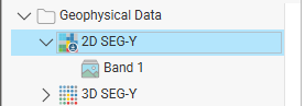
In the project tree, the file is organised into the main data object and the colour band object. Drag either one into the scene to view the data.

3D SEG-Y Data

Leapfrog Geo imports 3D SEG-Y data in *.segy and *.sgy formats.

To import 3D SEG-Y data, right-click on the Geophysical Data folder and select Import 3D SEG-Y. Leapfrog Geo will ask you to specify the file location. Click Open to start importing the file.

Leapfrog Geo will read the data in the file and match the data to the expected format. In most cases, Leapfrog Geo will set the correct values from the information in the file.

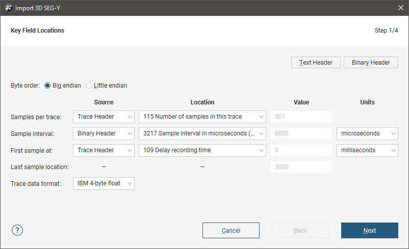
There are four steps to work through. In the last step, you can choose how many slices to import. First, set up the Key Field Locations. There are buttons at the top of the window for displaying the Text Header and Binary Header, which may be useful in deciding what import settings to use.

Settings for setting the Key Field Locations are:

• Byte order. This will be Big endian or Little endian and must be correct in order for the other data in the file to be read correctly.
• Samples per trace. This is the number of samples in each trace. If the correct value cannot be read from the file, you can set it manually by selecting User from the Source dropdown list.
• Sample interval. This is the vertical sample spacing for the trace data and is almost always stored in thousandths of true units. If the correct value cannot be read from the file, you can set it manually by selecting User from the Source dropdown list.
• First sample at. This is the delay recording time for the first sample. If the correct value cannot be read from the file, you can set it manually by selecting User from the Source dropdown list.
• Last sample location. This is read-only and is the calculated location from the last sample in the trace.
• Trace data format. This should be defined in the binary header.

Click Next to move on to setting the Coordinate Field Locations. In this step, the More button displays the trace header fields:

Settings for setting the Coordinate Field Locations are:

• Inline. This is the location in the trace header of the in-line coordinate.
• Crossline. This is the location of the cross-line location.
• X. This is the location of the X-coordinate of the trace location.
• Y. This is the location of the Y-coordinate of the trace location.
• Scalar. This the coordinate scale factor used for ground coordinates. It is read-only, but you can choose to disable the scalar by disabling the Apply scalar option.

Click Next to move on to setting the Tie Points. By default, these are calculated from the trace headers, but if they are not in the trace headers or if you have more precise values from the text header or from another source, click User supplied and entering these values manually.

The Spacing along Inlines and Spacing between Inlines fields are calculated from the specified tie points.

Click Next to move on to selecting the slices you will import. The Total column tells you the number of in-lines, cross-lines and z-slices that will be imported.

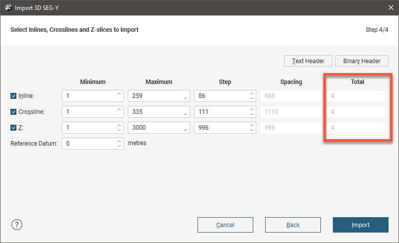
If you wish to import fewer or more slices, adjust the Minimum, Maximum or Step values, and the Total number of slices will be updated:

When you are finished, click Import. The file will appear in the Geophysical Data folder.

In the project tree, the file is organised into an extents object and separate folders for the in-lines, cross-lines and z-slices:

You can drag slices into the scene one-by-one or display, say, all z-slices by dragging the Z-slices folder into the scene.

To delete slices, right-click on them and click Delete.

If you wish to add more slices, right-click on the data object and select Import More Slices:

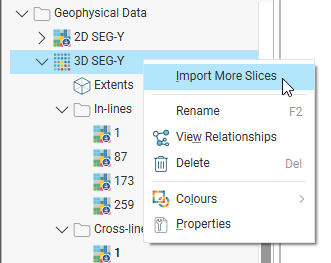
This launches the Import 3D SEG-Y window once again and you can select additional slices by changing the Minimum, Maximum or Step values in the last step.

ASEG_DFN Files

Leapfrog Geo imports ASEG_DFN points in *.dfn format. To import an ASEG_DFN file, right-click on the Geophysical Data folder and select Import ASEG_DFN. Leapfrog Geo will ask you to specify the file location. Click Open to import the file. In the window that appears, enter a name for the file, then click OK. Next set the X, Y and Z coordinates and click OK. If you select no column for the Z coordinates, all Z values will be set to zero.

The file will appear in the Geophysical Data folder.

UBC Grids

Leapfrog Geo imports UBC grids in *.msh format, together with numeric values in properties files in *.gra, *.sus, *.mag and *.den formats. UBC grids can be evaluated against geological and numeric models, which can then be exported with the grid.

Importing a UBC Grid

To import a UBC grid, right-click on the Geophysical Data folder and select Import UBC Model. In the window that appears, click Browse to locate the file to be imported. Click Add to add any properties file, although these are not required.

For any properties file, click the Inactive Value field to mark cells as inactive. Doing so does not change the data but ensures that cells with the inactive value can be hidden when the grid is displayed in the scene. If you do not set this value when importing the grid, you can set it later by double-clicking on the grid in the project tree.

Click Import. The grid will appear in the Geophysical Data folder.

Evaluating UBC Grids

UBC grids can be evaluated against geological and numeric models as described in Evaluations. However, UBC grids cannot be evaluated against fault blocks and mutli-domained RBF interpolants, although they can be evaluated against the parent geological model and the parent numeric model.

Mapping Category Evaluations

When a UBC grid is exported with a category evaluation, category data is mapped to an editable numeric value. You can edit this by double-clicking on the grid in the project tree, then clicking on the Export Mappings tab:

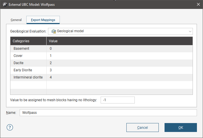
Change the numeric value assigned to each lithology, if required. You can also change the value assigned to blocks that have no lithology.

Exporting a UBC Grid

To export a UBC grid, right-click on it in the project tree and select Export. Select the evaluations to export with the grid, then select a folder. Click OK to export the grid.

A UBC grid can also be exported as points to a CSV file. To do this, right-click on the grid and select Export as Points. You will then be prompted to select a file name and location. Once you have clicked Save, select the CSV export options for null values and numeric precision, then click OK.

The CSV file will contain:

• X, Y and Z columns, which represent the centre of each grid block
• I, J and K columns, which is the grid block index. I is in the range 1 to NI, J is in the range 1 to NJ and K is in the range 1 to NK, where NI, NJ and NK are the grid dimensions.
• One or more data columns

GOCAD Models

To import a GOCAD model, right-click on the Geophysical Data folder and select Import GOCAD Model. Leapfrog Geo will ask you to specify the file location. Click Open to import the file.

In the window that appears, set the Subsample Rate and enter a Name for the model. Click OK to import the model, which will appear under the Geophysical Data folder.

You can then evaluate geological models, interpolants and distance functions in the project on the model. In the case of geological models, you can also combine two or more models to evaluate on the model. To evaluate a model, right-click on the model object in the project tree and select Evaluations. See Evaluations for more information.

A GOCAD model can be exported as points to a CSV file. To do this, right-click on the grid and select Export as Points. You will then be prompted to select a file name and location. Once you have clicked Save, select the CSV export options for null values and numeric precision, then click OK.

The CSV file will contain:

• X, Y and Z columns, which represent the centre of each grid block
• I, J and K columns, which is the grid block index. I is in the range 1 to NI, J is in the range 1 to NJ and K is in the range 1 to NK, where NI, NJ and NK are the grid dimensions.
• One or more data columns

Magnetotelluric Resistivity Files

Leapfrog Geo imports magnetotelluric resistivity (OUT) files in *.out, *.out.gz and *.mod formats. To import an OUT file, right-click on the Geophysical Data folder and select Import Magnetotelluric Resistivity Model. Leapfrog Geo will ask you to specify the file location. Click Open to import the file. In the window that appears, set the options required, then click OK to import the model. The model will appear under the Geophysical Data folder.

You can then evaluate any geological model, interpolant or distance function in the project on the model. In the case of geological models, you can also combine two or more models to evaluate on the model. To evaluate a geological model, interpolant or distance function, right-click on the model object in the project tree and select Evaluations. See Evaluations for more information.

A magnetotelluric resistivity grid can be exported as points to a CSV file. To do this, right-click on the grid and select Export as Points. You will then be prompted to select a file name and location. Once you have clicked Save, select the CSV export options for null values and numeric precision, then click OK.

The CSV file will contain:

• X, Y and Z columns, which represent the centre of each grid block
• I, J and K columns, which is the grid block index. I is in the range 1 to NI, J is in the range 1 to NJ and K is in the range 1 to NK, where NI, NJ and NK are the grid dimensions.
• One or more data columns

 

Got a question? Visit the Seequent forums or Seequent support