Block Models

The Block Models folder can be used to import and create block models. You can also create block models and sub-blocked models, which can then be exported for use in other applications. Creating block models within Leapfrog Geo has the advantage that the resolution can easily be changed.

Geological models and interpolants can be evaluated on block models as described in Evaluations. If you have the Leapfrog Edge extension, estimators can also be evaluated on block models. If you have the Hydrogeology extension, flow models can also be evaluated on block models.

The rest of this topic describes importing and creating block models in Leapfrog Geo, viewing block model statistics and exporting block models. It is divided into:

• Importing a Block Model
• Creating a Block Model
• Displaying a Block Model
• Viewing Block Model Statistics
• Exporting Block Models

Importing a Block Model

Leapfrog Geo imports block models in the following formats:

• CSV + Text Header (*.csv, *.csv.txt)
• CSV with Embedded Header (*.csv)

You will need to map the data in the file to the block model format Leapfrog Geo expects.

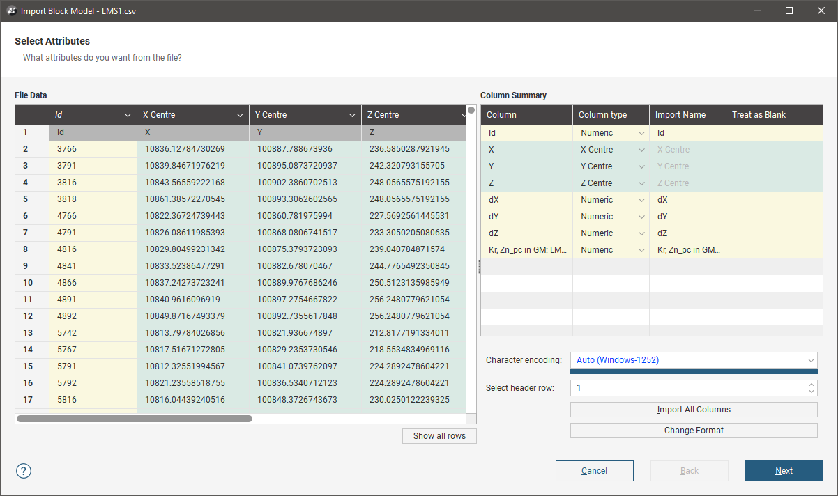
To import a block model in CSV format, right-click on the Block Models folder and select Import Block Model. Select the file you wish to import and click Open. An import window will be displayed in which you can map the columns in the file to those Leapfrog Geo expects. Once you have mapped the required columns, click Next to define the grid.

If you are opening a block model *.csv file created by Leapfrog, the Grid Definition fields will be automatically populated.

You can also enter the grid definition values manually.

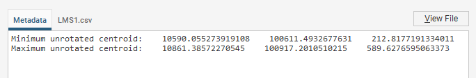
A Metadata tab contains additional information extracted or processed from the file content, including the minimum and maximum grid corners were the grid not rotated.

In cases where Leapfrog Geo cannot automatically parse the grid definition information from the file, it will be necessary to enter the block size, position and extent values for the block model you are importing. You may be able to find this information in the header at the top of the *.csv file, which is displayed on the right side of the screen. Copy the relevant information from the header into the Parent blocks, Sub-blocks and Position and Size fields.

Validation messages at the bottom of the Grid Definition fields check to see if the values in the Grid Definition fields result in a match for the blocks in the source file. Once you have a valid set of definition fields, the validation message will read: All the blocks in the file match the grid you've defined.

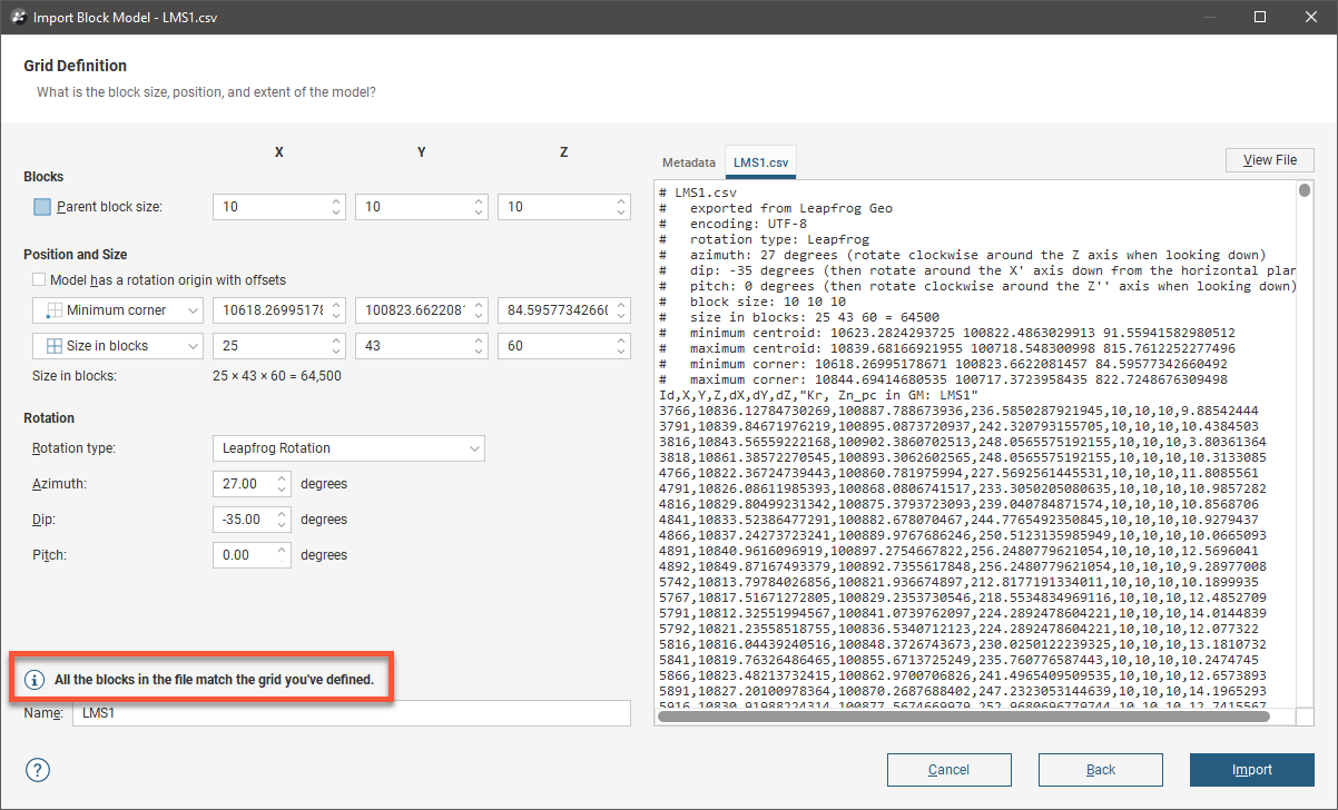
Click Finish. The block model will be imported and will appear in the Block Models folder.

To make this process easier, Leapfrog Geo makes it easy to move numbers from the file over into the Grid Definition fields. Select content from the right pane and drag it over to the Grid Definition fields. As you drag the value over fields on the left, boxes will be highlighted to show where the value(s) will be entered when you drop them. You may include the label and other content in the selection, and only the selected numbers will be pasted. When a line contains several numbers, all can be selected and dragged over, and depending on how many numbers you selected, two or three adjacent fields will be highlighted to show where the numbers will go.

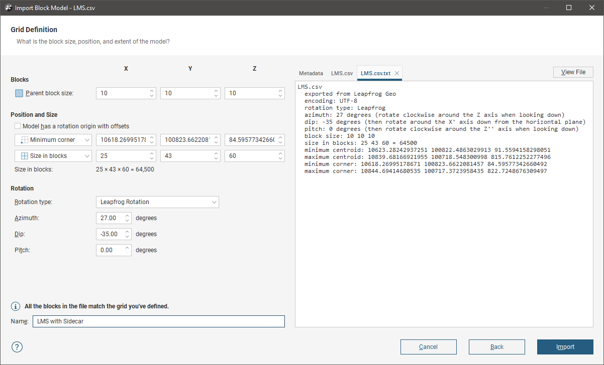
Some *.csv block model files do not have the file grid definition data in a header at the top of the file, but instead have the information in a second 'sidecar' file that accompanies the block model file. If no grid definition header is apparent for the file you have selected, check the source folder to see if there is another file that contains the grid definition information. If the block model was exported from Leapfrog Geo, the file will be named the same but also have “.txt” at the end. If Leapfrog Geo can identify the sidecar file it will be displayed in a tab on the right side of the window.

Some *.csv block model files may only have the origin coordinates in the header, or no definition at all. If it is possible, ask the source of the file you are using for the grid definition information used on the original block model; reconstructing the information will result in a similar but not the same block model.

Creating a Block Model

To create a new block model, right-click on the Block Models folder and select New Block Model. The New Block Model window will appear, together with a set of controls that will help you set the size, location and orientation of the model in the scene:

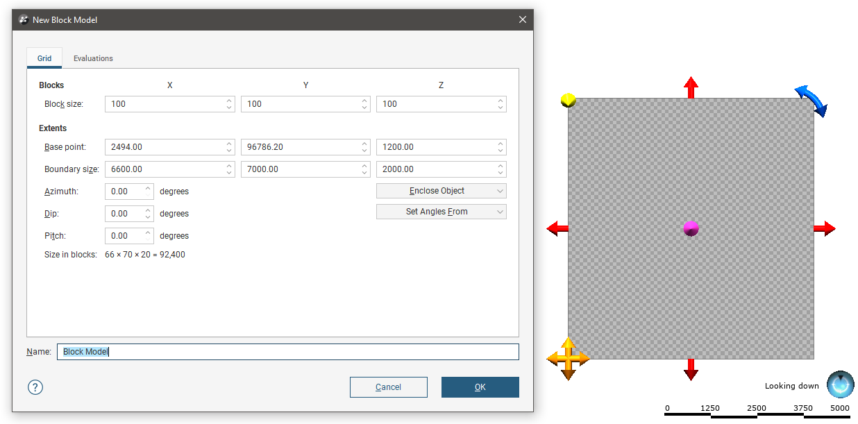
The block model is defined from its Base point, and the reference centroid is the Base point plus one half the Block size. Block models extents always include complete blocks, and when changes are made to the Block size parameter, the model’s extents will be enlarged to fit the Block size.

If you know the values you wish to use for the model’s Extents, enter them in New Block Model window. You can also:

• Use the controls in the scene to set the extents.
  • The orange handle sets the Base point.
  • The red handles adjusts the size of the boundary.
  • The blue handle adjusts the Azimuth.
• Use another object’s extents. Select the object from the Enclose Object list.

You can create a tilted block model by adjusting the Azimuth, Dip and Pitch angles, or you can Set Angles From the slicer or moving plane.

It is a good idea to use larger values for the Block size as processing time for large models can be considerable. Once you have created a block model, you can change its properties to provide more detail.

You can also evaluate the block model against geological models, interpolants and distance functions in the project. To do this, click on the Evaluations tab. All objects available in the project will be displayed. Move the models you wish to use into the Selected list.

Enter a Name for the block model and click OK. The model will appear under the Block Models folder. You can make changes to it by double-clicking on it.

Displaying a Block Model

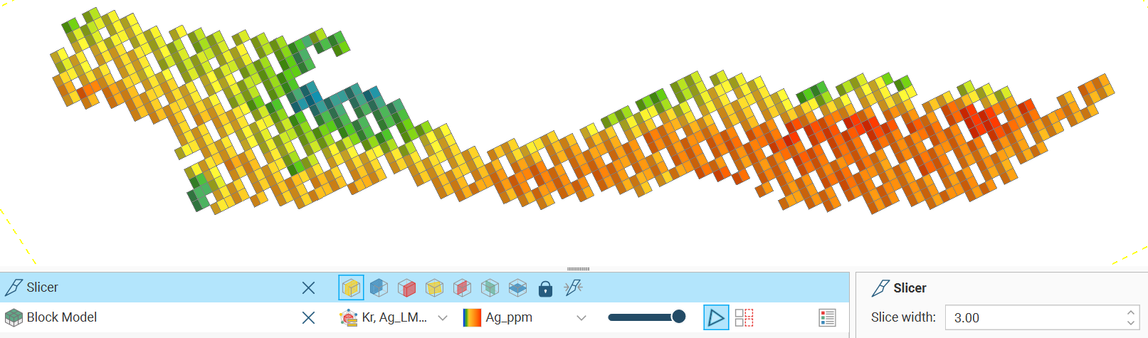
Along with the standard Slice mode options in the shape list properties panel for making sliced views of the block model, there is a 2D slice mode option. This option displays a regular block model or an octree sub-blocked block model at the surface of the slicer. It has several advantages over viewing a thick slice, where entire blocks may be missing or may be hidden by foreground blocks well in front of the slicer, depending on your slice thickness. Here, the display of a standard thick slice suggests there are holes in the block model, whereas in reality the centroids of those ‘missing’ blocks are outside of the thick slice and so not displayed:

When 2D slice mode is enabled, each block intersecting the slicer is depicted:

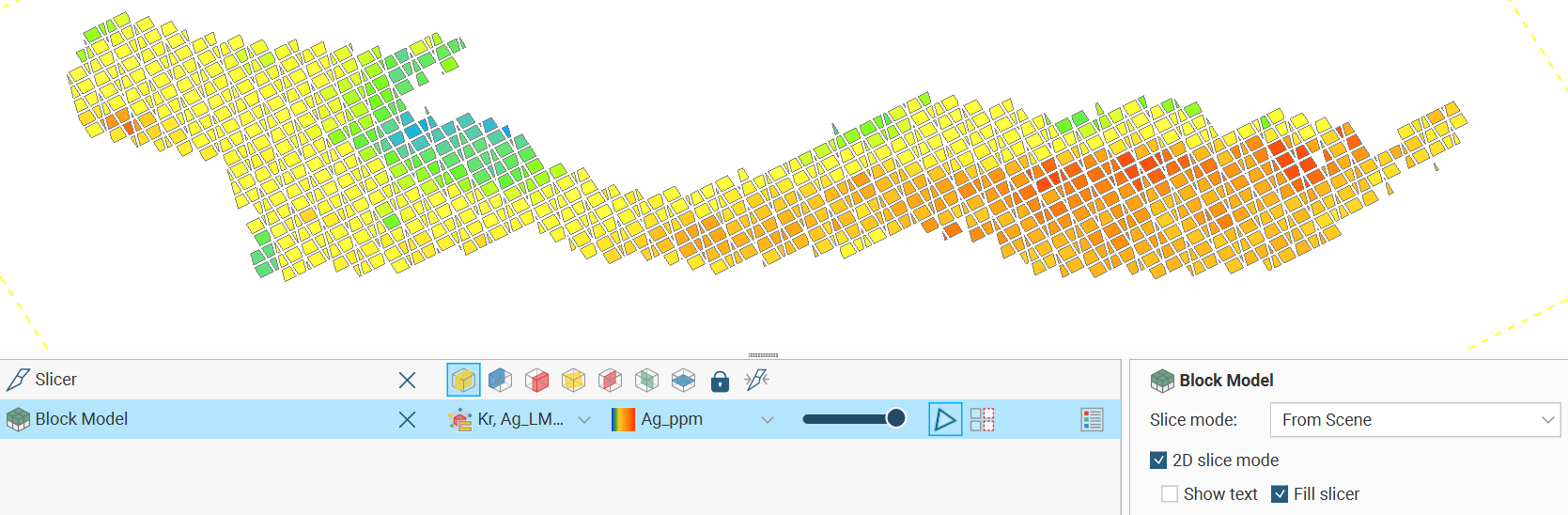
The Fill slicer option provides the choice between an outlined shape for the intersection of each block with the slicer, or a filled shape:

The Show text option provides the choice between seeing a value on screen for each block intersecting the slicer, or not. The default value is the value for the column selected to colour the block model:

Click the Format Display Text button to open the text format dialog in which you can customise the scene text displayed for each block, including the column values displayed and the colouring of different parts of the text label.

The size of the gap around a block can also be customised. Specify a fixed gap size to be used between all blocks, or choose a data column and the gap around each block will be proportional to the selected value of that column for the block. The selected value can also be the result of a calculation from Calculations and Filters. These variable gaps are created by scaling each block with a scaling factor between 0 and 1, linearly mapped from 0 to the selected attribute maximum.

Block models can also be added to a section layout where they will have an appearance similar to the 2D slice mode view. This presentation option includes a query filter and an index filter. See Section Layouts for more information on designing section layouts.

When a block model is displayed in the scene, there is a Query Filter option that includes filters created in Calculations and Filters:

When a block model is displayed in the scene, there is an Index Filter option for displaying the grid:

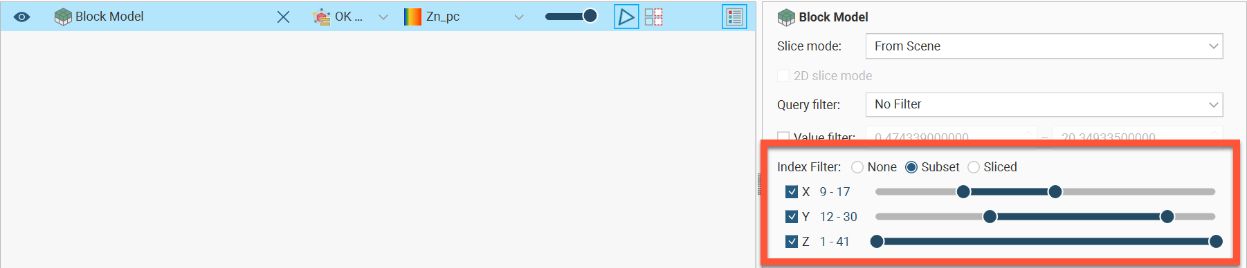
The Index Filter can be set to Subset or Sliced.

• Subset shows the union of the selected X, Y and Z ranges.
• Sliced shows the intersection of the selected X, Y and Z ranges.

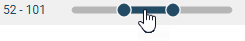
The range sliders have two modes: coarse control and fine control. Here an index filter is used for a set of values that ranges from 1 to 160; it is displayed in dark blue, to show the full range of values in coarse control mode:

You can restrict the data displayed by dragging on the handles. Here the range of values is restricted to 1 to 50:

You can click and drag on the selected range to change the values displayed:

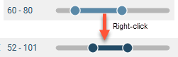
To switch to fine control, double-click anywhere along the range slider. Here the range of 52-101 has been expanded along the whole slider, giving you more control over the position of the range end points:

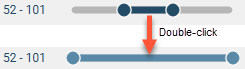
The slider is displayed in light blue in fine control mode.

Now you can use the handles to further restrict the range displayed:

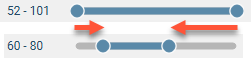
Right-click on the slider to return to coarse control and the full range of values. Here, right-clicking reverts to coarse control, with the range restricted to the original range of 52-101:

Viewing Block Model Statistics

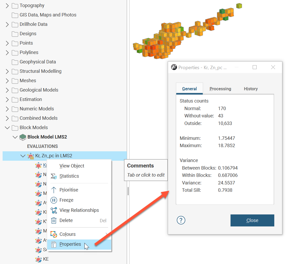
To view statistics on a block model, right-click on the model in the project tree and select Statistics. The following options are available:

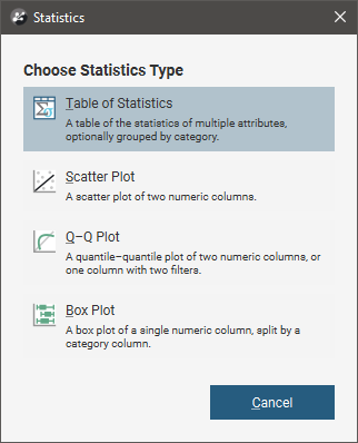
See the Statistics topic for more information on each option:

• Table of Statistics
• Scatter Plots
• Q-Q Plots
• Box Plots

Right-clicking a block model evaluation or a numeric calculation and selecting Statistics opens a univariate graph for the selection. See Univariate Graphs in the Statistics topic for more information.

Table of Statistics

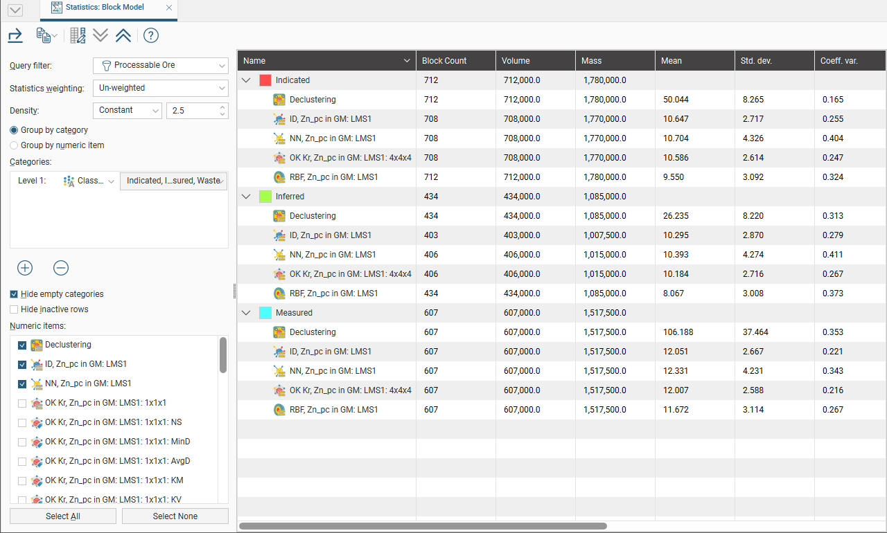
You can view statistics for all evaluations and calculations made on a block model broken down into categories and organised by numeric evaluations and calculations. To view statistics, right-click on a block model in the project tree, select Statistics then select the Table of Statistics option.

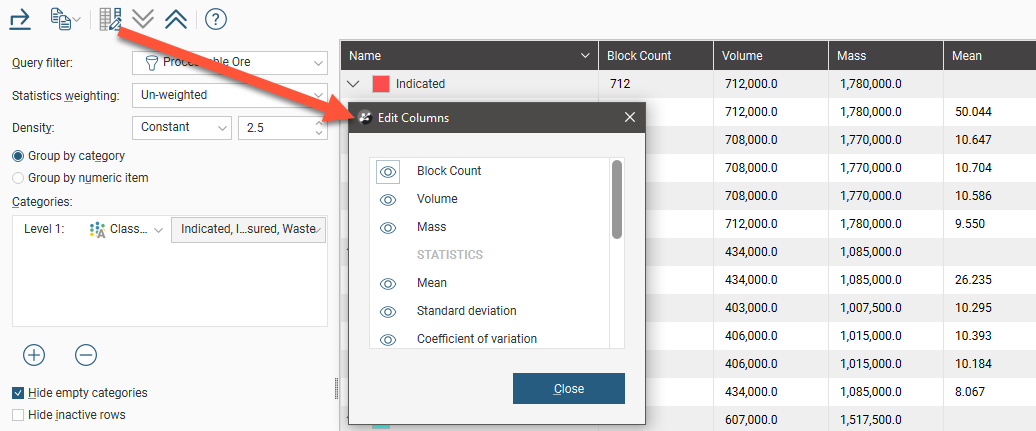
You can view statistics for as many numeric and category columns as you wish. When you have at least one Category column selected, you can organise the information displayed in two ways: Group by Category or Group by Numeric. Here, statistics are displayed organised by the category data columns:

The Query filter option uses a related filter to constrain the data set to a selected subset.

Statistics can be unweighted, weighted by volume or weighted by tonnage. Select the option you require from the Statistics weighting list.

You can also set the Density to be a Constant value that you specify, or you can use the one of the columns in the table.

The Categories list provides category classification options. When selected, the set of statistics measures for each evaluation or numeric calculation will be shown for each category.

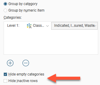
You can hide empty categories (those with a count of zero) and inactive rows using the options below the Categories list:

Group by category and Group by numeric column provide options for the table organisation. You can also change what columns are displayed in the table by clicking the Edit columns button (). This opens a window in which you can select the columns that are displayed in the table:

Click rows to select them, and select multiple rows by holding down the Shift or Ctrl key while clicking rows. You can then copy rows by clicking the Copy button (), which allows you to copy the selected row(s) or all rows in the table.

The arrow buttons quickly expand () or collapse () rows.

Separately, the block model evaluation object has a Properties window with useful statistics. One important section is the Variance section, providing the variance Between Blocks and Within Blocks, useful for calculations applying Krige’s Relationship and determining the variance correction factor and block dispersion variance.

Exporting Block Models

Block models created in Leapfrog Geo can be exported in the following formats:

• CSV + Text Header (*.csv, *.csv.txt)
• CSV with Embedded Header (*.csv)
• CSV as points (*.csv)
• Surpac Block Model Files (*.mdl)
• Datamine Block Model Files (*.dm)

To export a block model, right-click on the block model in the project tree and select Export. You will be prompted to select the file format.

Enter a name and location for the file and click Save. Next, you will be able to choose custom settings for the selected format.

The rest of this topic provides more information about exporting block models in CSV, Datamine and Surpac formats.

 

Got a question? Visit the Seequent forums or Seequent support
© 2022 Bentley Systems, Incorporated