
Conditional Simulation
The features described in this topic are only available if you have the Leapfrog Edge extension and are subscribed to Seequent Evo. Conditional simulation utilises a Seequent Evo cloud processing service.
There are two methods in common use for conditional simulation of continuous numeric variables: Sequential Gaussian Simulation and Turning Bands. Both methods are capable of producing ensembles of realisations that reproduce the desired characteristics in a conditional simulation: Reproduction of the histogram and variogram while honouring the sample data values.
Leapfrog Geo uses the Turning Bands methodology in conditional simulation. Turning Bands can be very highly parallelised. Sequential methodologies have been historically preferred due to computing constraints limiting the number of bands that could be applied using Turning Bands, leading to visible artefacts in the realisations. We can now leverage the availability of distributed parallel computing resources to make rapid simulation generation possible employing the Turning Bands methodology.
The Turning Bands method involves two distinct steps:
- Generate a set of non-conditional simulations that can reproduce the histogram and variogram. Turning Bands generates a one-dimensional simulation of values along a line, such that the covariance model is reproduced along that line. When repeated multiple times on randomly oriented lines over a sufficiently large volume, the sum of the one-dimensional simulations produces a three-dimensional reproduction of the input distribution and covariance model.
- The resultant non-conditional simulation is then post-processed or ‘conditioned’ to the input data locations using a Kriging estimation step.
Conditional simulation results in an evaluation that generates a new set of output columns on a block model.
In Leapfrog Geo, there are two steps in evaluating a conditional simulation onto a block model:
- First, create a conditional simulation estimator. This is a container for the input data links and the conditional simulation parameters. No simulation is involved at this stage.
- Next, evaluate the conditional simulation estimator onto a block model.
It is at the second stage that Leapfrog Geo will connect to Seequent Evo computational services to access cloud resources and run the simulation computations, as follows:
- Publish geoscience data objects to the selected Seequent Evo workspace
- Execute several processing tasks using Seequent Evo cloud computing resources
- Import requested simulation outputs back into the Leapfrog Geo block model as new columns
- Present a validation report
When the simulation is complete, Leapfrog Geo will update the block models locally.
The rest of this topic describes:
- Prerequisites
- Creating a Conditional Simulation Estimator
- Running a Conditional Simulation
- Reviewing Conditional Simulation Results
- Viewing Validation Reports
- Comparing Individual Simulations
Prerequisites
Prior to creating a conditional simulation, these prerequisite steps need to be completed.
Defining a suitable domain is the initial step for any simulation or estimation in Leapfrog Geo.
The decisions you make with respect to stationarity when defining the domain are more significant for simulation than they are for estimation.
- Estimation is relatively tolerant of trends in grade and variability. Grade only needs to be stationary at the scale of the search neighbourhood, which permits local averaging to be performed.
- Simulation is a global method that aims to reproduce the histogram and the variogram for the input data. It does this by application of a spatial monte-carlo sampling from the global (declustered) histogram of samples. This requires that there should be no systematic trends in mean grade or the variogram, i.e. no second order stationarity.
In practice, however, natural phenomena such as grades always show some trend in mean/variance, particularly towards the margins of the deposit. Defining the domain to minimise this and maximise stationarity will improve simulation results.
Conditional simulation in Leapfrog Geo is intended for use with dense regular sampling, such as in grade control. In this scenario, trends are less important, and conditioning is usually sufficient to mitigate the effect and ensure reasonable local reproduction.
To maximise the quality of your conditional simulation results, consider these factors when you are domaining:
- Respect sharp boundaries such as faults and strong lithological control.
- Consider variations in data density.
- Consider large variations in local mean grade.
Underground grade control is generally highly clustered, as fanned drilling is dictated by the constrained platforms from which drilling can be conducted. Declustering this data is very important in creating a spatially representative cumulative distribution function, as this is the distribution from which simulated values are drawn.
Declustering should be used to determine a set of appropriate declustering weights. For more information, see the Sample Geometries (Declustering Objects) topic. Declustering weights are exported along with data values to Evo.
Open-pit grade control sampling is typically conducted on a regularly-spaced grid pattern, and declustering is not usually necessary.
Normal score values are required to model a normal scores variogram. To create a normal score values object, right-click on the values object under the domained estimation object, then select Transform Values. A new values object with the same name will be added to the domained estimation object, appended with NS.
Normal score values from Leapfrog Geo are not published to Evo. Instead, raw values with declustering weights are published. Normal score transformation with de-spiking is performed in Evo.
Conditional simulation requires a variogram modelled on normal score values. Create a new transform variogram model by right-clicking on the Spatial Models folder and choosing the New Transformed Variogram Model option.
For more information on modelling the transformed variogram, see the Transform Variography topic.
Creating a Conditional Simulation Estimator
Right-click on the Estimators folder in the domained estimation and select New Conditional Simulation.
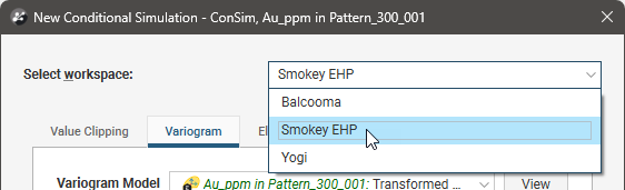
Choose a Seequent Evo workspace from the Select workspace dropdown list.
Conditional simulation is not supported by combined estimators.
Value Clipping
Use the Value Clipping tab to constrain the data values used in the dataset, discarding outliers. In most cases it should not be necessary to clip values.
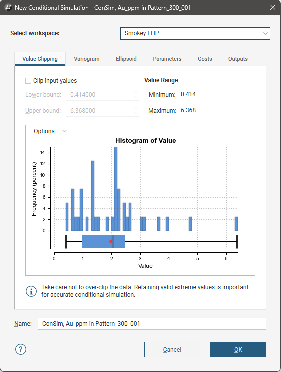
Not overclipping data is important for accurate conditional simulation as extreme valid values are relevant to the simulation. Correct statistical reproduction of high grade values is of critical importance. Instead of clipping off outliers, all the data should be retained unless there are sound reasons for clipping input values.
Variogram
In the Variogram tab, select the transformed variogram model and the declustering object to use in the conditional simulation.
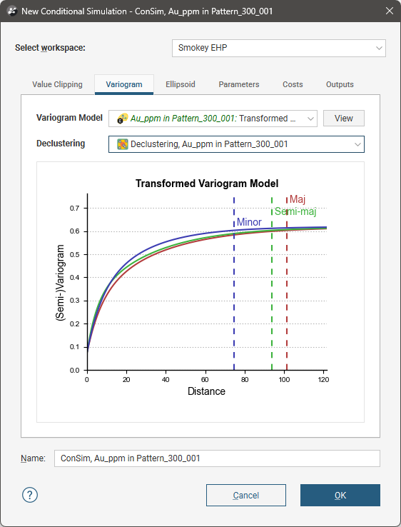
Leapfrog Geo does not enforce that normal score variograms have a sill of 1. In general, if a variogram stabilizes at a different value, it is an indication that the domain is not stationary.
If the selected transformed variogram has a total sill less than 1, conditional simulation will normalise the variogram, rescaling the transformed variogram so that the total sill is equal to 1. This is to guarantee accuracy of the conditional simulation result, as without the rescaled function there is a risk of high-grade values not being reproduced in the outputs.
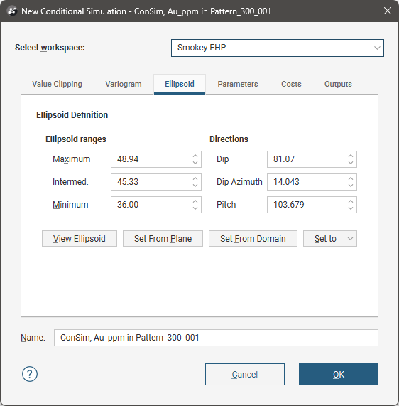
Ellipsoid
The Ellipsoid tab defines the primary anisotropic search volume size and orientation. Neighbourhood samples will be selected from within this search volume.
Parameters
The Parameters tab contains additional parameters relevant to the conditional simulation.
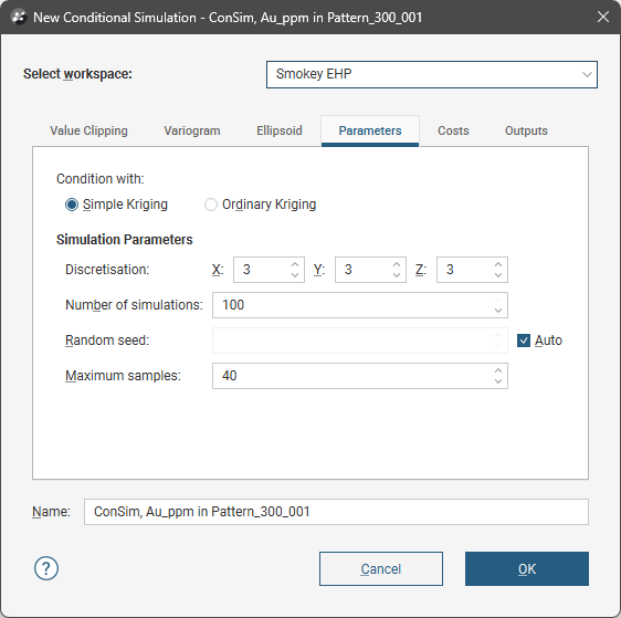
Two options are provided to Condition with: Simple Kriging and Ordinary Kriging.
Simple Kriging is the default option, and should be the preferred selection. Conditional simulation is a global method that makes a strong assumption of stationarity. Simple Kriging requires a similarly strong assumption. Simple Kriging calculates weights for local samples based on the variogram, and also includes a term for the weight given to the mean. As the relevance of local samples decreases and as the samples become less correlated to the target, the weight attached to the mean correspondingly increases. As a result, simulated grades revert towards the mean away from sampling. Beyond the range of influence of the variogram, simulations revert to non-conditional with an expected value that is the declustered mean of the dataset.
Ordinary Kriging is provided as an option in case locally precise results are preferred despite higher variability and the risk of potential bias. The mean reverting behaviour of simple Kriging may contradict the expected behaviour of grades in the real world, and the results can be visually jarring. When this is the case, it may be preferable to condition simulations with ordinary Kriging, which assumes that the neighbourhood samples inform the local mean adequately. However, the reproduction of the variogram may be distorted, as the simulated grades will incorporate trend, which can artificially inflate spatial variance. A simulation conditioned by ordinary Kriging will revert to non-conditional when no samples are found inside the search ellipsoid. When using ordinary Kriging, use a search that is large enough to ensure that peripheral blocks still find a sufficient number of neighbours.
Simple Kriging should be preferred over ordinary Kriging as ordinary Kriging can lead to higher variability and potential bias.
When assessing variogram reproduction, focus on the reproduction at ranges shorter than the variogram range.
Discretisation sets the number of discretisation points in the X, Y and Z directions. To take account of block support, each block is broken down (discretised) using a point grid for each block for simulation, before averaging point values back up to the block scale. When specifying a discretisation grid, there should be sufficient nodes per block to produce a reliable estimate of the average grade in the block per realisation.
The point grid is a transient data object and is not preserved. The simulated values for each point are not retained.
Set the X, Y and Z parameters to 1 for no discretisation, with a single centroid point per block.
Choose the Number of simulations to be generated. The maximum of 100 is also the default option.
You can specify a Random seed value to be used by the pseudo-random number generator used in the simulation. If you leave the Auto box ticked, each time the simulation is run, different values will be created by the pseudo-random number generator and the simulations will exhibit effectively random variations between simulations. However, if you need reliably repeatable results across simulation executions, this can be forced by specifying a fixed Random seed value.
If you need to repeat a simulation that has already been run using an Auto random seed, look in the validation report to find the seed that was used and enter that seed value into Random seed for subsequent executions.
The Maximum samples threshold limits the number of samples used in a search neighbourhood. The maximum number of samples used in a neighbourhood is the sole parameter exposed for operational control that is associated with the Turning Bands algorithm. When compared with the Sequential Gaussian Simulation method, Turning Bands is less sensitive to the neighbourhood, i.e. to the number of initial samples included in the search relative to the number of previously simulated nodes. What is being estimated with Turning Bands during the conditioning step are the residuals between the actual data at sample locations and the simulated values at sample locations.
The default value has been selected to be a reasonable value to use in most cases. As a general principle, variogram models with low continuity can be conditioned with a larger neighbourhood, while models with high continuity will require fewer neighbours for conditioning. However, test alternative values before committing, as the results of changing the number of maximum samples can be counter-intuitive.
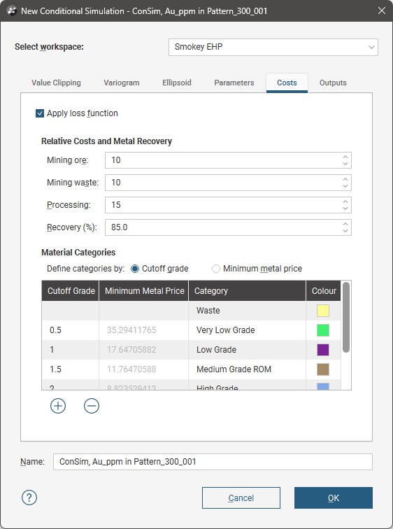
Costs
In an open pit mine, all material must be moved and therefore a choice must be made about the destination of all material: run of mine ore, stockpiles or waste. We cannot know in advance the actual grade of any block and must base decisions on an estimate. Those estimates are always imperfect, and so there is the inevitable risk of misclassification:
- Rock that is actually ore may be sent to the waste dump.
- Rock that is actually waste may be sent to the mill.
Both these types of misclassification result in loss, but the losses incurred are asymmetric: the economic loss resulting from sending ore to the waste dump is not the same as the loss from sending waste to the processing plant.
There is also uncertainty about the actual grade of the block, but the magnitude of loss incurred depends on actual grade.
An economic classification function is used to account for both this asymmetry in losses and also the underlying uncertainty in grade. This is achieved by applying a loss minimisation function to all realisations of a simulation ensemble.
In the Costs tab, enable Apply loss function to add profitability to the simulation.
Set the specific cost values for Mining ore, Mining waste, and ore Processing, using the currency and units of mass used in the project, e.g. USD$25/tonne. The expected Recovery percentage from processing is also needed.
There are two options for Material Categories:
- Cutoff grade. Category classifications are defined based on grades.
- Minimum metal price. Category classifications are defined based on minimum metal price. Prices used will depend on the units used in estimation, e.g. if commodity grades are estimated in g/t then the commodity price should be expressed in $/g; if commodity grades are estimated in %, then the commodity price should be expressed in $/t.
Click the Add button (![]() ) for a new table row in which a Category can be identified along with the associated Cutoff Grade or Minimum Metal Price. Click the colour chips to change the associated colour for the category, if required.
) for a new table row in which a Category can be identified along with the associated Cutoff Grade or Minimum Metal Price. Click the colour chips to change the associated colour for the category, if required.
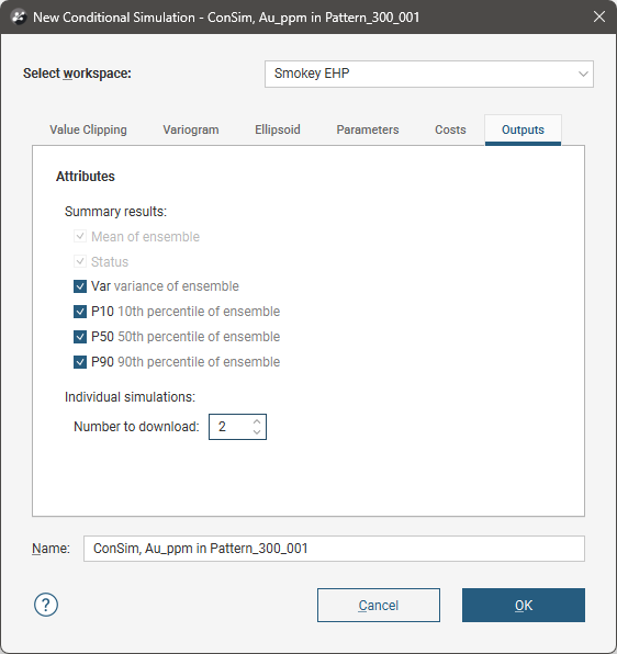
Outputs
Conditional simulation will always produce the Mean of ensemble and Status results per block; simulated blocks will have a Status of Normal. You can also generate additional results, although these are optional:
- Var (variance of ensemble). The statistical variance across the simulated result values.
- P10 (10th percentile of ensemble). The statistical 10th percentile point in the simulated result values.
- P50 (50th percentile of ensemble). The statistical 50th percentile point in the simulated result values.
- P90 (90th percentile of ensemble). The statistical 90th percentile point in the simulated result values.
If the dataset has a normal distribution, P50 is the same as the median value, but P50 is the preferred measure for central tendency when the distribution is not normal or not known.
Under Individual simulations, Number to download specifies how many simulations you want returned for inspection from the Evo processing service. You do not need to have any simulations returned, but obtaining a sample allows for inspection of the results for validation and verification. It is also not usually necessary to download all the simulations for inspection. The simulations returned will be randomly selected from the ensemble, although the name assigned will always be sequentially numbered to simplify the use of these realisations in user-defined calculations.
Running a Conditional Simulation
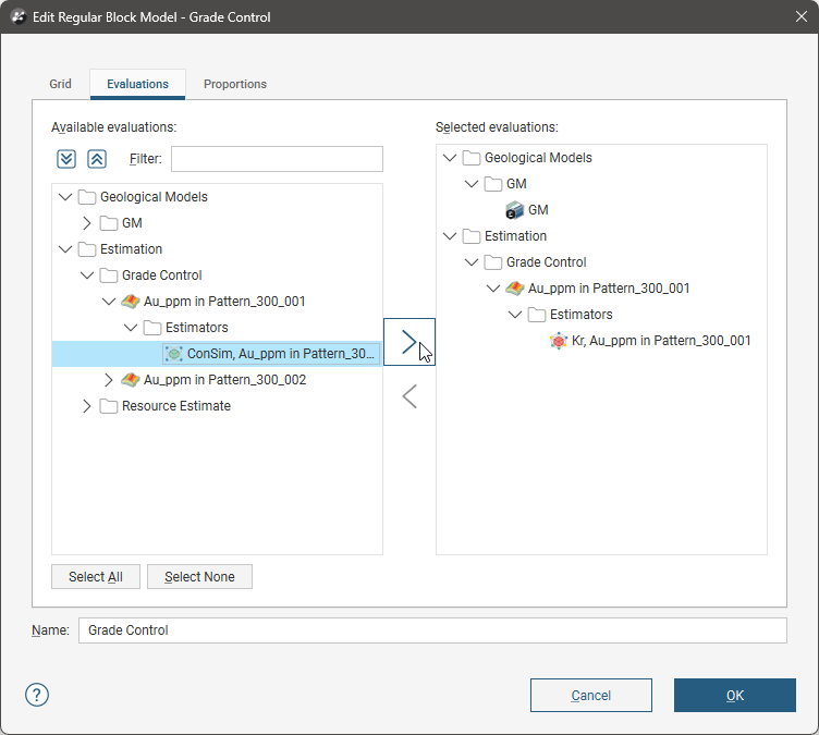
To run a conditional simulation, right-click on a regular block model in the project tree. Select Evaluations and add the conditional simulation estimator to the block model.
Conditional simulation is not supported for octree sub-blocked models, fully sub-blocked models, or variable-z block models.
When you click OK, Leapfrog Geo will connect to Seequent Evo computation services to access cloud resources and run the simulation computations. How long this process takes will depend on the number of points in the dataset. Progress will be shown in the Leapfrog Geo processing queue.
Publishing Geoscience Data Objects to Evo
Initially, Leapfrog Geo will publish some geoscience data objects to the selected Evo workspace:
- Composited raw grade data as XYZ points, with declustering weights
- The normal scores variogram model
- Target grid nodes from the regular block model
While normal scores values are calculated in Leapfrog Geo for the purposes of modelling a normal scores variogram, only raw values are published to Seequent Evo. Normal score transformation of the raw data, with de-spiking, will be performed as part of the cloud processing in Evo.
Breaking Ties (De-spiking)
In many datasets, particularly lower grade gold deposits, it is common to have repeated values. There are nearly always multiple values at the lower level of detection, but repeats of other values are also common. We say that these values are ‘tied’, like when competitors in a game get the same score. In that case, a process is used to ‘break the tie’ in the game, to determine a revised score for the competitors so they are not stuck with the same score.
Conditional simulation relies on converting raw grade values into equivalent values from a Gaussian distribution and then back-transforming simulated Gaussian values into equivalent raw grades.
The process of breaking ties in the data ensures the data used in the simulation smoothly fits a normal distribution instead of having spikes in the histogram at points due to systemic assaying factors. The process of breaking ties adds a small component of random noise to repeated values in a deterministic way, such that the process is repeatable.
Data Transformation
The raw data values published by Leapfrog Geo to Evo are transformed into normal score values.
A continuous distribution function is created to transform raw data values to equivalent Gaussian values. The continuous distribution function models the forward and backward transformation, and is called whenever data values are transformed in either direction. Transformation uses the declustered values provided by Leapfrog Geo, to ensure that the normal scores histogram is spatially representative.
Non-conditional Simulation
Seequent Evo cloud computing resources will generate a non-conditional simulation across the grid Zunc(u)
The underlying point scale grid defined from the specified discretisation parameters will be used, generating values for each point such that the simulated grid values reproduce the histogram and variogram. This is repeated to create an ensemble of simulation results, up to the Number of simulations specified.
Conditioning
The non-conditional simulations then undergo Kriging conditioning:
- Evaluate the unconditional realisation at data locations, and with the evaluated values as data, perform Kriging of the grid Z*unc(u)
- Subtract to obtain the residual field for all grid locations r(u) = Zunc(u)- Z*unc(u)
- Perform Kriging on the grid using actual sample values Z*(u)
- Add the residual field to the Kriging map Z(u) = Z*(u) + R(u)
Back-Transformation to Blocks
At this point, the ensemble simulation data is normalised data associated with the underlying discretised grid of points. What happens next is:
- Simulated values are back-transformed into the raw data space.
- Point simulations are averaged to block support, per realisation.
There will then be some additional post-processing to calculate ensemble statistics per block.
Validation Processes
When the main Turning Bands block conditional simulation is being executed, there will also be a simultaneous execution of a sub-set of validation simulations.
In this validation task, a set of point scale simulations are created on the centroids of the target block model, and these are used to validate the reproduction of the input distribution (using summary statistics and continuous distribution function plots) and the variogram in normal score space.
Return Simulation Outputs to Block Model
Once the simulation process is complete, simulation outputs are returned back into the Leapfrog Geo block model as a new set of columns.
Present Validation Report
Validation results are added to the project tree for inspection.
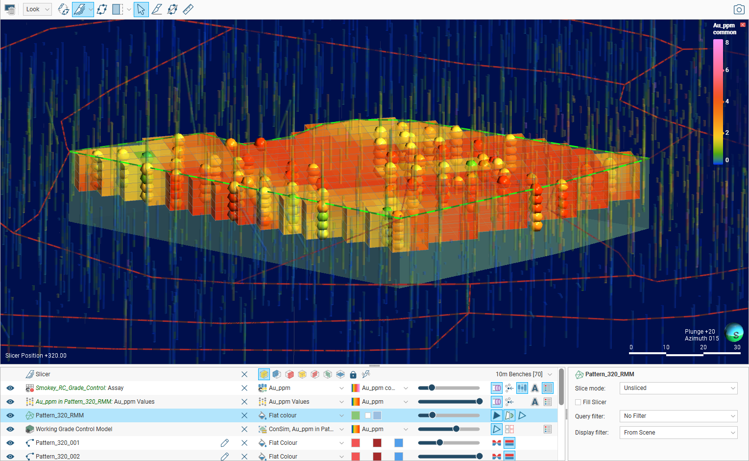
Reviewing Conditional Simulation Results
Review the resultant grade estimate in the scene alongside the input sample values:
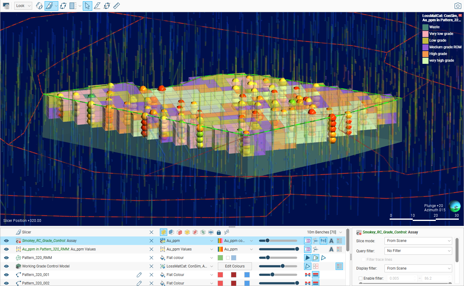
If it was enabled, you can also review the calculated loss function value categories for optimum material classification based on the grade uncertainty:
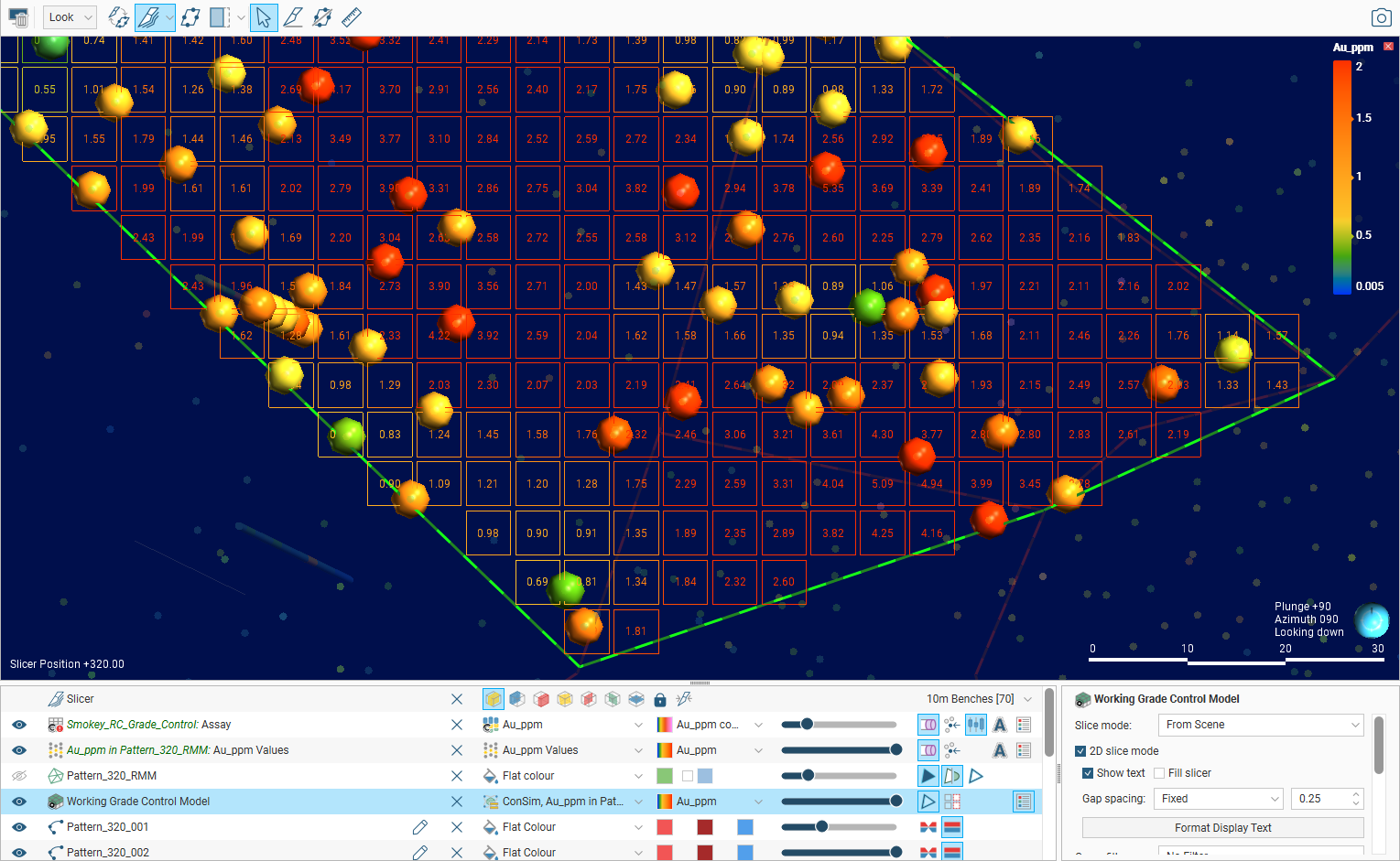
You may find it useful to view the block model in 2D with text labels:
We recommend using shared colourmaps for standardisation and clear communication. For more, see Colour Options in the Visualising Data topic.
Viewing Validation Reports
Validation reports generated from a conditional simulation will be added to the block model in the project tree under the heading Consim Reports. Right-click on a report and select Open in Seequent Evo to open it in your browser:
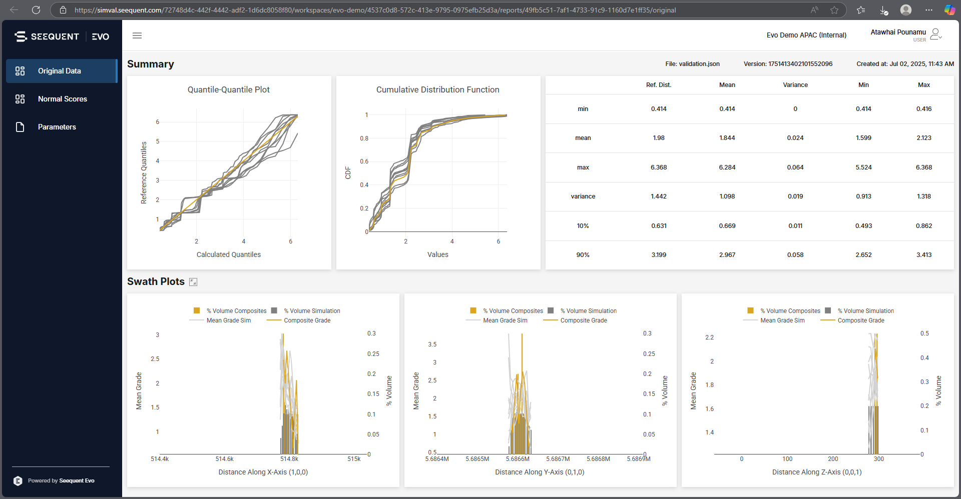
Switch between the Original Data and the Normal Scores views using the sidebar.
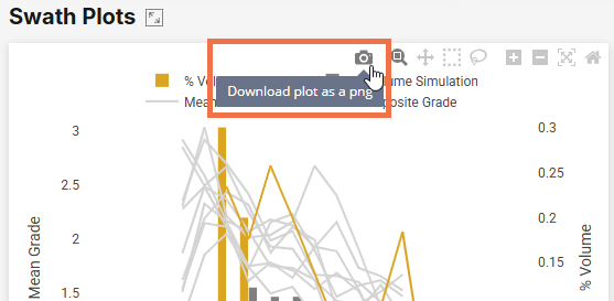
Hold your mouse cursor over a chart to reveal a toolbar.
From the toolbar, you can save each chart as a local PNG file by clicking the camera button:
To reframe a chart around a region of interest, click the magnify button, then click-and-drag a box around the region of interest:
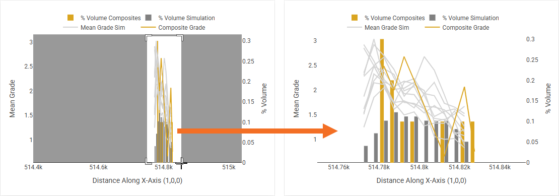
There are also controls for panning and zooming in and out. Each of the axes can be dragged to be repositioned.
To reset the chart to the original appearance, there are Autoscale and Reset axes buttons.
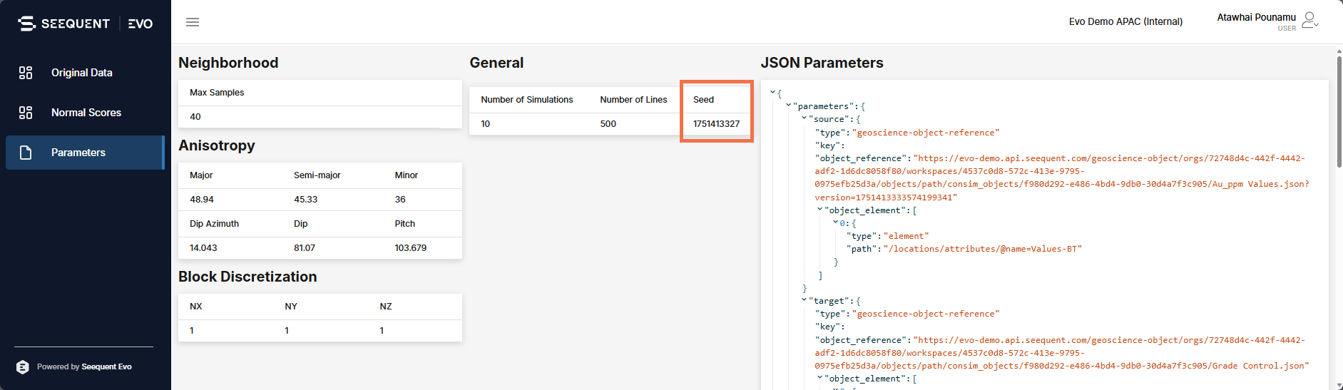
Select Parameters in the sidebar to see a report of the parameters used to generate the conditional simulation, including the JSON parameters used by the Seequent Evo simulation service. One particularly useful detail in the report is the identification of the Seed used. See Parameters above to see how this number can be used in the Random seed input parameter field to get repeatability in results.
Comparing Individual Simulations
If you specified any number of individual simulations to download, each individual simulation can be selected as colouring options in the shape list for the conditional simulation:
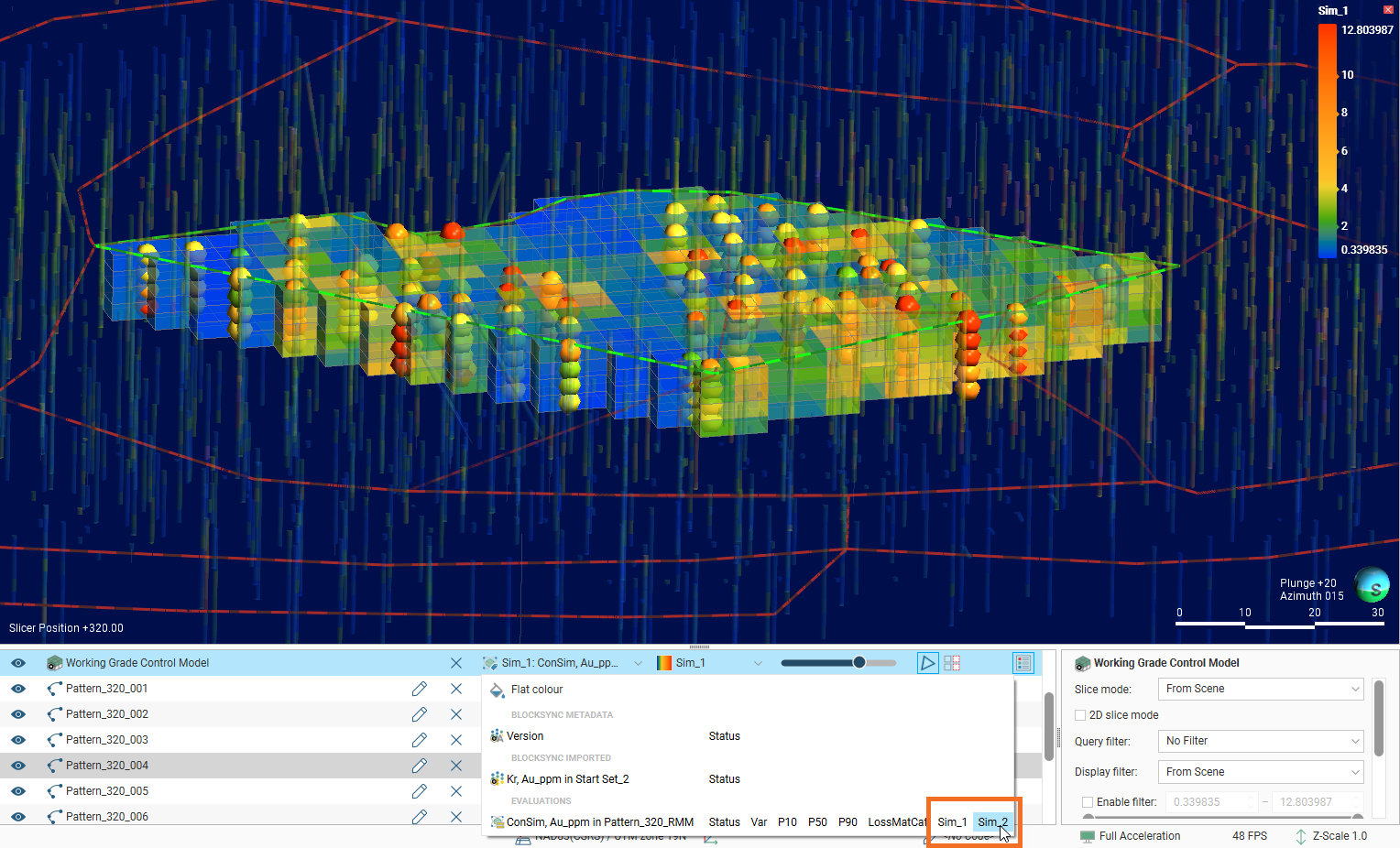
Switch between individual simulations to obtain an impression of the similarities between simulation runs.