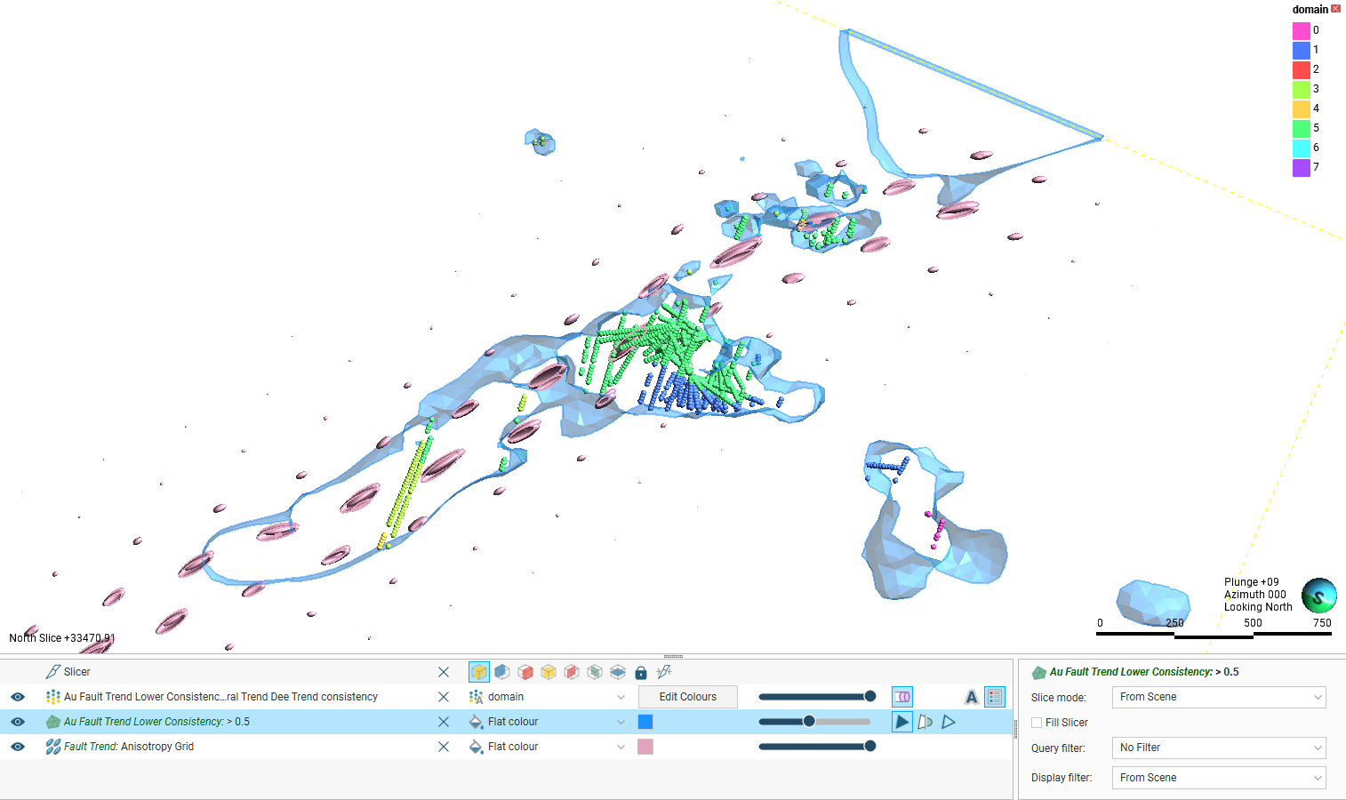
Building a Structural Trend
Structural trends can be constructed using structural data disks, lineations, meshes and triaxial ellipsoids. Most of these data objects can be created manually. Triaxial ellipsoids are a unique type of data generated by Driver. Driver can also create the other structural data types Leapfrog Geo can use to derive structural trends. Using Driver to create the structural data inputs provides a fast, probabilistic and repeatable way to obtain structural data directly from drilling data.
For more information on the Leapfrog Geo Driver integration, see the Driver Integration topic.
The following descriptive anisotropy parameters are important concepts when creating structural trends:
- The Strength parameter describes how much stronger the trend is in the maximum and intermediate plane than in the minimum direction.
- The Range distance exponentially decreases the input structural data influence.
Different strategies and algorithms are used to produce different structural trends and apply them to interpolations, but the basic process is as follows:
- A continuous structural trend function is derived from the structural data inputs.
- When interpolating, local input data is progressively divided into mini-clusters with input data points that have similar anisotropy, constrained by a limit set within the structural trend. Depending on the algorithm being used, this might be enhanced by geometric partitioning, which segments the region of interest into sections for consideration.
- Next in the interpolation process, adjacent mini-clusters are combined into clusters no larger than the maximum permitted, while preserving consistent anisotropy.
- Finally, the interpolation process derives an interpolant and uses that to produce isosurfaces, using the structural trend and interpolation parameters to infer the values between data points.
Creating a Structural Trend
To create a new structural trend, right-click on the Structural Trends folder (in the Structural Modelling folder) and select New Structural Trend. The New Structural Trend type selection window will appear:
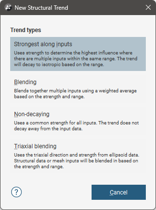
There are four structural trend types:
Each of these is described in detail below.
Strongest Along Inputs
Where a trend is isolated to a region near documented structures and the influence away from the structures decreases and the trend away from data is isotropic, Strongest along inputs can represent the decreasing influence away from the input data.
Near the input data, the Strength and Range values will inform the structural trend. Where multiple inputs in the same range exist, the relative influence of each is determined by their respective Strength values.
Beyond the range set for the input data, the trend will decay towards isotropic.
It is possible to set a non-isotropic global mean trend for a Strongest Along Inputs type, however this will result in the same outcome as if the type had been set to Blending. If there is an anisotropic global mean trend, choose the Blending type instead of Strongest Along Inputs.
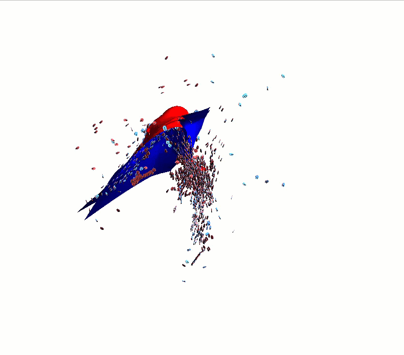
Meshes and structural data disks were used to generate a Strongest Along Inputs structural trend. The meshes have a strength of 2 and the structural data disks have a strength of 5.
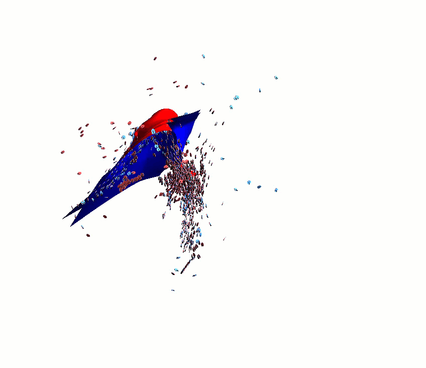
Note that where the trend approaches an isotopic trend, no ellipsoid is visualised.
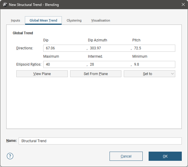
Blending
Where a trend is isolated to a region near documented structures and the influence away from the structure decreases and the global mean trend is anisotropic, Blending can represent the decreasing influence away from the input data.
Near the input data, the Strength and Range values will inform the structural trend. Where multiple inputs in the same range exist, the relative influence of each is determined by a weighted average of both the Strength and Range of each component trend input.
Beyond the range set for the input data, the trend will decay towards the anisotropic global mean trend.
It is possible to specify that the global mean trend is isotropic, but consider the use of the type Strongest Along Inputs in this situation instead.
Meshes and structural data disks were used to generate a Blending structural trend. The meshes have a strength of 2 and the structural data disks have a strength of 5. A global mean trend of 3:3:1 was applied using a plane drawn vertically down the scene in the middle.
Non-decaying
The Non-decaying structural trend type should be selected when it can be assumed that the strength of the trend does not decay as you get further away from the input data. This is useful when the geology has a fairly constant trend across the model, but with some directional shift.
Where multiple inputs exist, the relative influence of each is determined by weighted averages derived from their respective Strength values. There is no Range parameter for the Non-decaying structural trend type.
There is no reduction in trend strength as distance increases from the input data.
Meshes and structural data disks were used to generate a Non-decaying structural trend. All inputs have the same strength of 5.
Triaxial Blending
When the structural data inputs include imported triaxial ellipsoidal trend data, alone or along with other structural trend inputs, use the Triaxial Blending structural trend type.
Triaxial Blending uses ellipsoidal trend data imported into Leapfrog Geo, and for each point described by an ellipsoid, taking the relative strengths in each of the three directional axes along with the trend direction information, simplifying and blending the data into a representative structural trend.
Beyond the range set for the input data, the trend will decay towards an automatically calculated global mean trend.
Trend ellipsoids generated from the data by Driver were imported and used to generate a Triaxial Blending structural trend. A filter was applied to the inputs to only use ellipsoids with a confidence over 0.5. A Minimum cluster size of 5 and a Maximum cluster size of 50 were specified.
Once you click on a structural trend type, the new Structural Trend window will open. Strongest along inputs, Non-decaying and Triaxial Blending have a window with three tabs, Blending has a slightly different window with four tabs.
The window for all new structural trend types will have an Inputs tab.
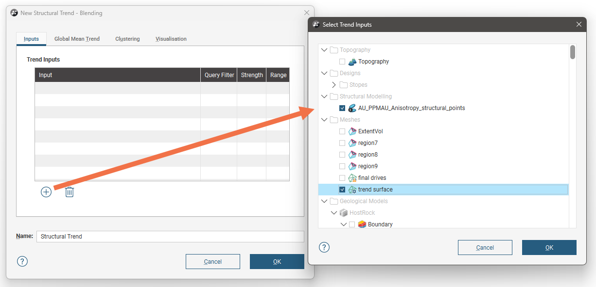
Clicking on the Select inputs(![]() ) button will open a window that shows the available data objects that can be used to inform structural trends. Select all that are required and click on OK. They will be added to the Trend Inputs list. Each input could have the following parameters:
) button will open a window that shows the available data objects that can be used to inform structural trends. Select all that are required and click on OK. They will be added to the Trend Inputs list. Each input could have the following parameters:
- For some data types, a Query Filter can be used to constrain the data used by applying a pre-existing filter. This is the only parameter that can be set for triaxial trend ellipsoids. If a query filter cell is blank, no filter can be applied for that data object. If a filter can be applied but none are available, No filter available will be displayed.
- The Strength parameter describes how much stronger the trend is in the maximum and intermediate plane than in the minimum direction.
- The Range distance exponentially decreases the input structural data influence. Range is not available for Non-decaying structural trends.
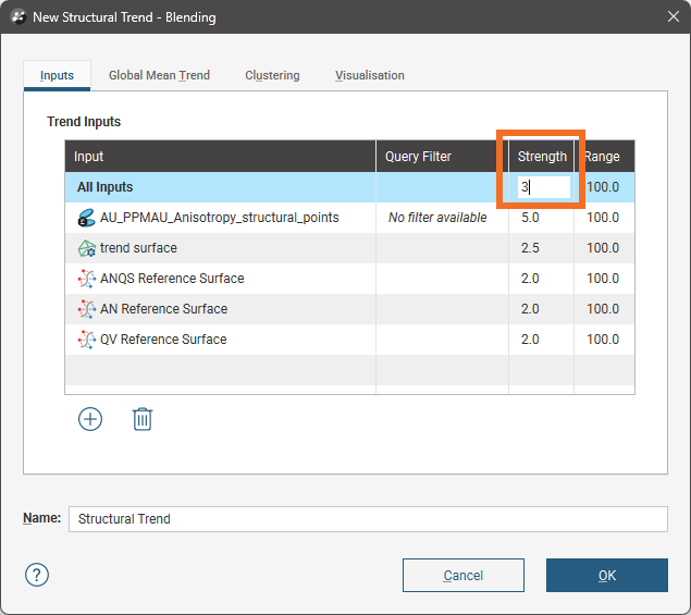
Use the All Inputs row to quickly set the Strength or Range values for all the listed inputs to the same values.
For Blending structural trend types, the Global Mean Trend tab allows you to specify the trend away from the structural trend that the model should tend towards. Maximum, intermediate and minimum ellipsoid ratios can be specified, and dip, dip azimuth and pitch directions.
You can enter the trend manually or add the moving plane to the scene and set the trend using the moving plane, as described in Setting a Global Trend.
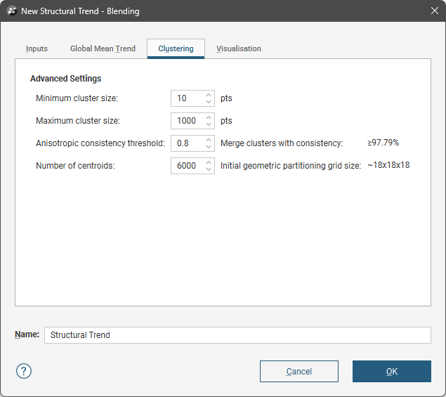
The Clustering tab settings are provided for adjustment of the structural trend algorithm behaviour. For Strongest along inputs, Blending, and Non-decaying, the tab appears as follows. Note that Minimum cluster size and Maximum cluster size are specified in number of input data points, and there is a parameter for Number of centroids:
For triaxial blending, the tab appears as follows. Note that Minimum cluster size and Maximum cluster size are specified as a percentage of the total number of input data points available:
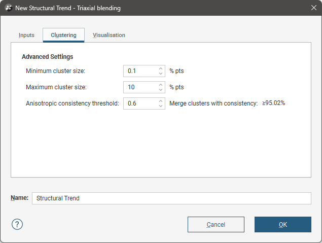
Minimum cluster size and Maximum cluster size constrain how the interpolation algorithm infers clusters when applying the structural trend. During structural trend clustering, the data points are clustered into small regions down as far as the minimum cluster size. These mini-clusters are then merged into larger clusters if the mini-clusters are sufficiently consistent in their respective anisotropies, up to the maximum cluster size. It cannot define clusters containing fewer data points than the minimum cluster size, and the cluster cannot have data points exceeding the maximum cluster size.
The Anisotropic consistency threshold controls how similar clusters need to be to be in order to be merged into a larger cluster.
Strongest along inputs, Blending and Non-decaying structural trend types have an additional algorithm parameter, Number of centroids, specifying how many centroids are in a three-dimensional initial geometric partitioning grid. The approximate number of centroids along each axis of the resulting grid is described by the Initial geometric partitioning grid size shown in the window. This initial geometric partitioning grid is not the visualisation grid defined on the Visualisation tab. Rather, this initial geometric partitioning grid is created in the interpolation process while clustering the data. The data inputs are broken down into the initial geometric partitioning grid’s cellular units as a primitive step, from which the clusters are then constructed, merged and simplified. This initial geometric partitioning grid cannot be viewed in the scene.
Increasing the number of centroids will result in a more stable model output when more input data is added to the interpolant using the structural trend, especially if that data causes the extents to change. However, more centroids will also mean that it is more likely that isolated regions might be harder to link to other regions, despite an obvious trend implying that the regions are probably connected. This can be aggravated by a large Minimum cluster size that forces the initial mini-clusters to enclose all the points in a grid cell, which could also result in adjacent mini-clusters being sufficiently inconsistent in anisotropy that they cannot link up into consolidated clusters.
Reducing the Number of centroids and the resolution of the initial geometric partitioning grid may contribute to being able to model these as connected regions. However, reducing the Number of centroids too much could result in significant impacts on parts of the model distant from a region where new data is added.
Otherwise, if your model is producing many small isolated interpolated surfaces you expect should be consolidating due to an obvious trend, you might try one or a combination of the following:
- Increasing the Maximum cluster size
- Decreasing the Consistency threshold
This may produce a result closer to what you expect. Similarly, if a model is producing large consolidated interpolated surfaces that you expect could be described better using multiple smaller regions, one or a combination of the following could drive the algorithm to infer this expectation:
- Decreasing Maximum cluster size
- Increasing the Consistency threshold
Changing the Minimum cluster size may also contribute in both cases, but a direct relationship cannot be stated. The larger the minimum cluster size, the less the local structural inputs will have influence. Increasing the minimum cluster size will combine more points into initial mini-clusters, and this may contribute to consolidating surfaces, but if the minimum cluster size is too high and the Number of centroids is too high, a counter-productive effect can result in inconsistent clusters that cannot be merged.
As a guiding rule of thumb, using a minimum cluster size of 1% the number of points, and a maximum cluster size of 10% the number of points will often produce good results.
As you adjust these clustering parameters, use caution and watch for patterns or artefacts that the adjustments provoke in the isosurfaces produced by interpolants. You may also need to adjust the Strength of the anisotropy to achieve a geologically sensible result. For a helpful workflow that will show the effect of the clustering parameters, see below.
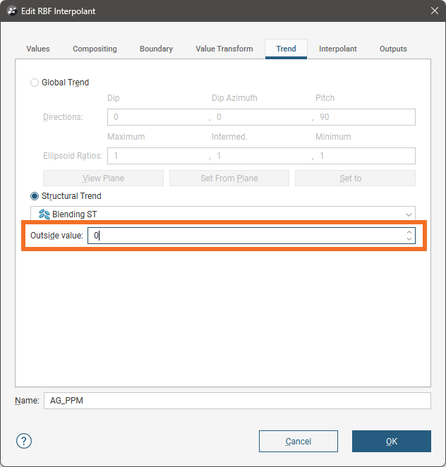
A separate parameter Outside value, associated with the interpolant, can also have an impact on the shape of the surfaces produced, and may also need to be adjusted in association with these structural trend parameters. Outside value sets the expected background value for the region. For more information, look for the help on the Trend tab for the interpolant in use.
The structural trend that is created can be viewed in the scene as a 3-dimensional grid of ellipsoids. The Visualisation tab provides for some customisation for this visualisation of the trend.
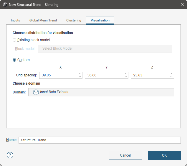
If Existing block model is selected and an available block model is chosen, an ellipsoid will be represented at the centroid of each block or sub-block in the block model.
If Custom is selected, ellipsoids will be spaced apart using the X, Y and Z Grid spacing distances within the Domain extents you specify.
Although the trend is represented in the scene using these ellipsoids, the trend is continuous between the representative ellipsoids in the three-dimensional grid. If you duplicate the trend and adjust the Grid spacing on the copy to shorter distances to get a higher-resolution grid, you can observe the same trend in the scene, but presented in higher detail.
Cluster Visualisation
Before altering these parameters, check how the interpolant clustered the data points. This will provide you insight that will be useful to determine how you might adjust the parameters.
Right-click on the structural trend object under an interpolant in the project tree, and select Extract Clusters to Points.
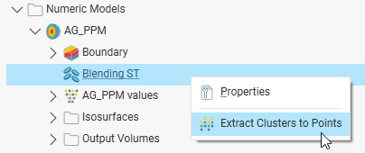
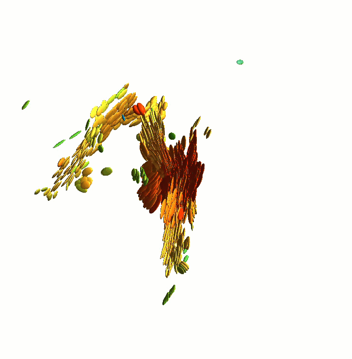
This will add a new object to the Points folder in the project tree. When added to the scene, this will show the points with different colours being used for each cluster identified.
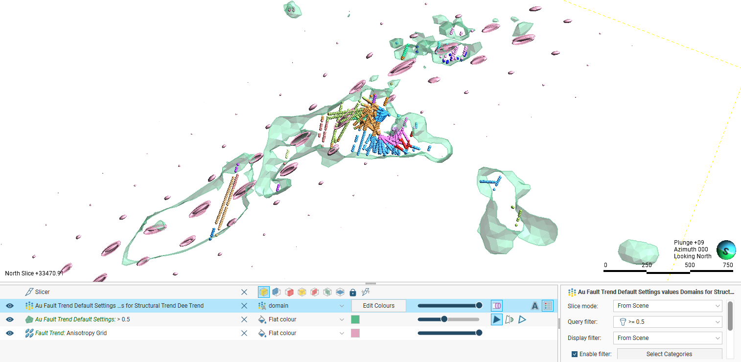
Based upon how the points have been clustered, you may choose to adjust the structural trend’s parameters, such as minimum or maximum cluster size. In this case, the Consistency threshold has been reduced from 0.8, as used above, to 0.4. Note how there are fewer clusters and more points with the same colour in close proximity, and the isosurface regions are more contiguous.