Interpolant Functions
Leapfrog Geo’s powerful 3D interpolation engine can interpolate any numeric data (e.g. ore grade or piezometric head measurements) to describe how a real, numerical quantity varies in three dimensional space. Interpolation produces an estimate or “interpolated value” of a quantity that is not known at a point of interest but is known at other points.
The simplest way to estimate values is to take the average of known values. Using this method, estimated values are the same everywhere, regardless of the distance from known data. However, this is not ideal as it is reasonable to assume that an estimated value will be more heavily influenced by nearby known values than by those that are further away. The estimates for unknown points when varying the distance from known point values is controlled by the interpolant function. Any interpolation function and the various parameters that can be set for each will produce a model that fits all the known values, but they will produce different estimates for the unknown points. It is important to select interpolation functions and parameters that make geologic sense. It may be necessary to identify a location that models predict differently, and plan drillholes to identify the best fit option.
Leapfrog Geo uses two main interpolant functions:
The Spheroidal Interpolant Function
In common cases, including when modelling most metallic ores, there is a finite range beyond which the influence of the data should fall to zero. The spheriodal interpolant function can be used when modelling in these cases.
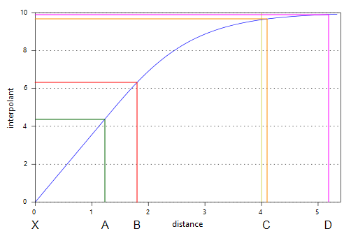
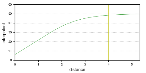
The spheroidal interpolant function closely resembles a spherical variogram, which has a fixed range beyond which the value is the constant sill. Similarly, the spheroidal interpolant function flattens out when the distance from X is greater than a defined distance, the range. At the range, the function value is 96% of the sill with no nugget, and beyond the range the function asymptotically approaches the sill. The chart below labels the y-axis interpolant. A high value on this axis represents a greater uncertainty relating to the known value, given its distance from X. Another way to think of this is that higher values on this axis represent a decreasing weight given to the known value.
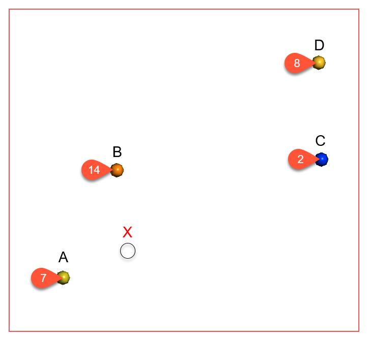
Known values within the range are weighted proportionally to the distance from X. Known values further from X than the range will all be given approximately the same weight, and have about the same influence on the unknown value. Here, points A and B are near X and so have the greatest influence on the estimated value of point X. Points C and D, however, are outside the range, which puts them on the flat part of the spheroidal interpolant curve; they have roughly the same influence on the value of X, and both have significantly less influence than A or B:
The parameters used to define a spheroidal interpolant are Total Sill, Nugget, Nugget to Total Sill Ratio, Base Range, Alpha, Drift and Accuracy.
To edit the parameters for an interpolant, double-click on the interpolant in the project tree and click on the Interpolant tab. The graph on the tab shows how the interpolant function values vary with distance and is updated as you change interpolant parameters:
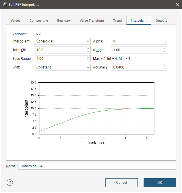
The yellow line indicates the Base Range. For this interpolant, the value of the interpolant is offset by the value of Nugget.
Total Sill
The Total Sill defines the upper limit of the spheroidal interpolant function, where there ceases to be any correlation between values. A spherical variogram reaches the sill at the range and stays there for increasing distances beyond the range. A spheroidal interpolant approaches the sill near the range, and approaches it asymptotically for increasing distances beyond the range. The distinction is insignificant.
Nugget
The Nugget represents a local anomaly in sampled values, one that is substantially different from what would be predicted at that point, based on the surrounding data. Increasing the value of Nugget effectively places more emphasis on the average values of surrounding samples and less on the actual data point, and can be used to reduce noise caused by inaccurately measured samples.
Nugget to Total Sill Ratio
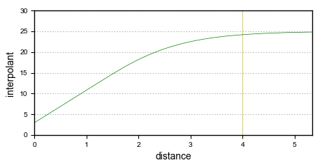
It is the Nugget to Total Sill ratio that determines the shape of the interpolant function. Multiplying both these parameters by the same constant will result in an identical interpolant. Here, the interpolant on the left has a nugget of 3 and a sill of 25; the one on the right has a nugget of 6 and a sill of 50. Note that because the nugget and sill have been increased by the same factor, the function has the same shape.
Base Range
The Base Range is the distance at which the interpolant value is 96% of the Total Sill, with no Nugget. The Base Range should be set to a distance that is not significantly less or greater than the distance between drillholes, so it can reach between them. As a rule of thumb, it may be set to approximately twice the average distance between drillholes.
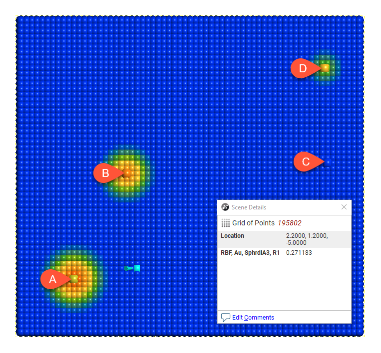
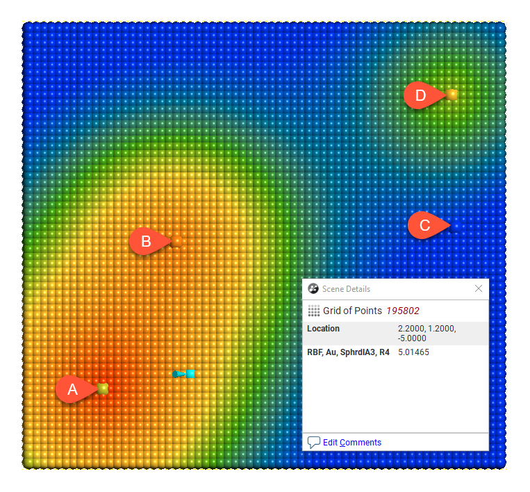
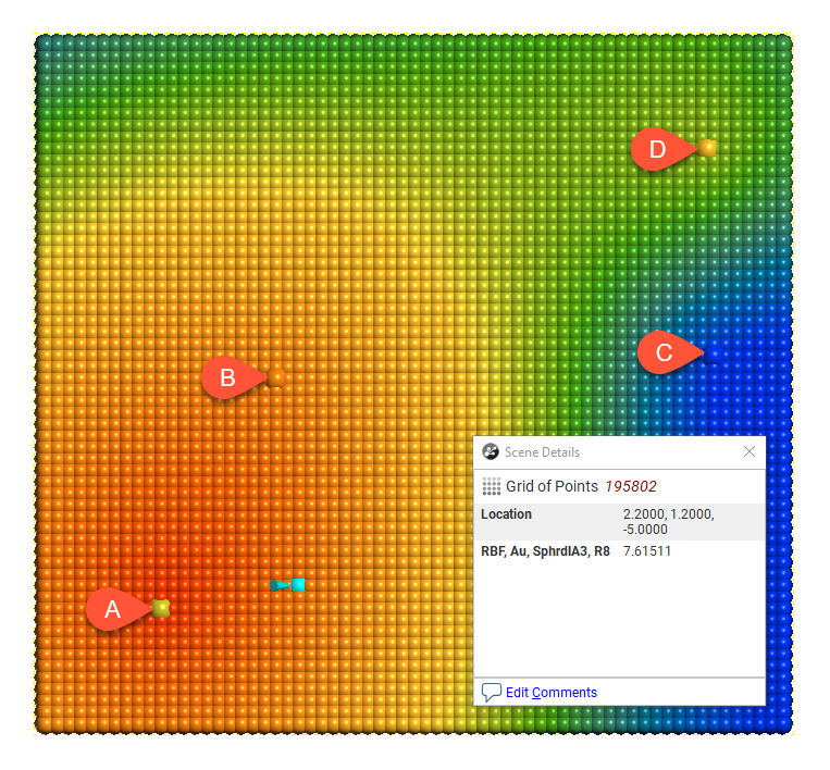
Here the effect of different range settings on the value of X is demonstrated using our trivial example of four drillholes:
Range = 1
Range = 4
Range = 8
Range = 30
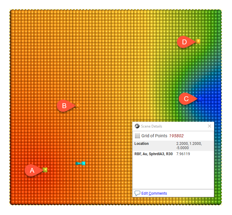
When the range is set to 1, it is too small to describe any real effect between drillholes. When the range is set to 30, distant drillholes have more influence, increasing the spatial continuity. Also illustrated is the range set to approximately the average distance between drillholes (range = 4) and the range set to about twice the average distance between drillholes (range = 8). Of these, the range set to 8 might be the best choice.
Alpha
The Alpha constant determines how steeply the interpolant rises toward the Total Sill. A low Alpha value will produce an interpolant function that rises more steeply than a high Alpha value. A high Alpha value gives points at intermediate distances more weighting, compared to lower Alpha values. This figure charts an interpolant function for each alpha setting, using a nugget of 8, sill of 28, and range of 5000. A spherical variogram function is included for comparative purposes. The inset provides a detailed view near the intersection of the sill and range.
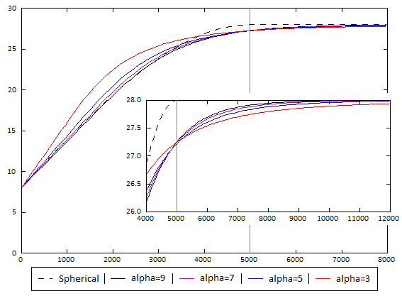
An alpha of 9 provides the curve that is closest in shape to a spherical variogram. In ideal situations, it would probably be the first choice; however, high alpha values require more computation and processing time, as more complex approximation calculations are required. A smaller value for alpha will result in shorter times to evaluate the interpolant.
The following demonstrates the difference between alpha = 3 and alpha = 9:
Alpha = 3
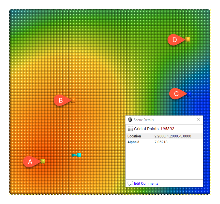
Alpha = 9
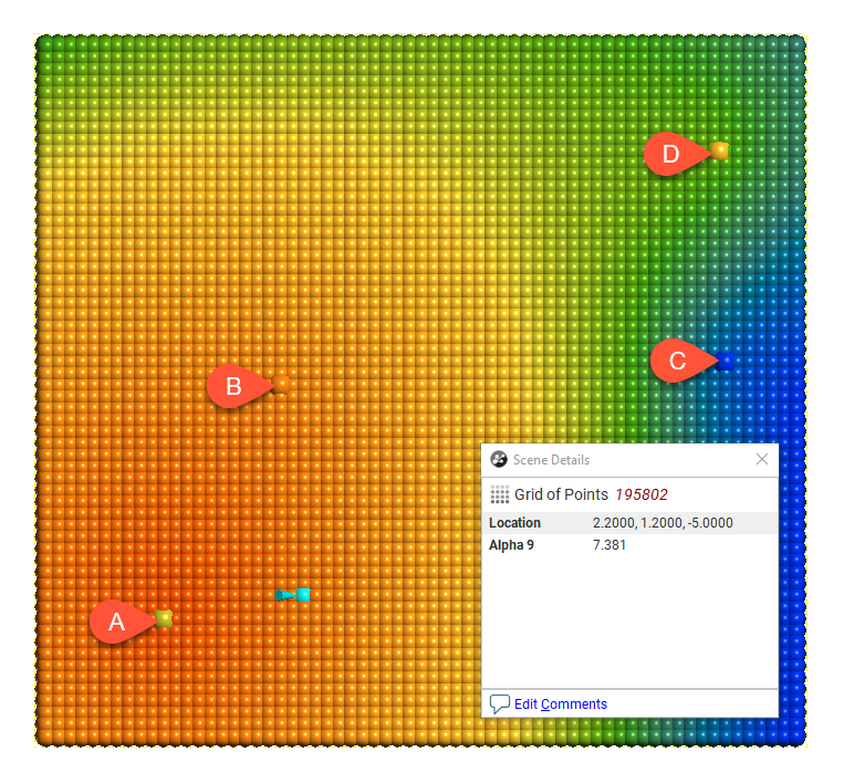
There is a measurable difference between the estimates at the point being examined, but for many purposes, using a lower alpha will result in satisfactory estimates and reduced processing time.
The effect of the alpha parameter on the spheroidal interpolant in Leapfrog Geo is different to the effect of the alpha parameter in Leapfrog Mining 2.x. If Alpha is set to 9 in Leapfrog Geo, the range corresponds to the range in Leapfrog Mining 2.x. To convert from Leapfrog Mining 2.x to Leapfrog Geo where the alpha is not 9, apply the following scale factors to the Leapfrog Mining 2.x range value to find the corresponding range in Leapfrog Geo:
| Alpha | Scale factor |
|---|---|
| 3 | 1.39 |
| 5 | 1.11 |
| 7 | 1.03 |
For example, if in a Leapfrog Mining 2.x project, the alpha is 5 for a range of 100, the corresponding range in Leapfrog Geo will be 111.
Drift
The Drift is a model of the value distribution away from data. It determines the behaviour a long way from sampled data.
- Constant: The interpolant goes to the approximated declustered mean of the data.
- Linear: The interpolant behaves linearly away from data, which may result in negative values.
- None: The interpolant pulls down to zero away from data.
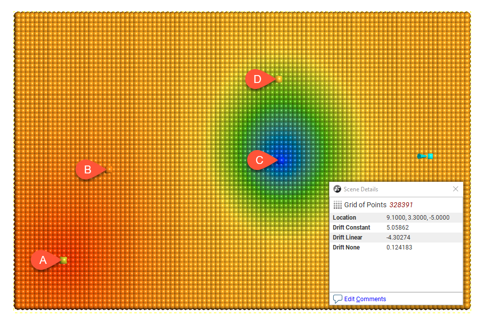
Here, the three Drift options for the interpolant are shown evaluated on grids:
Drift = Constant
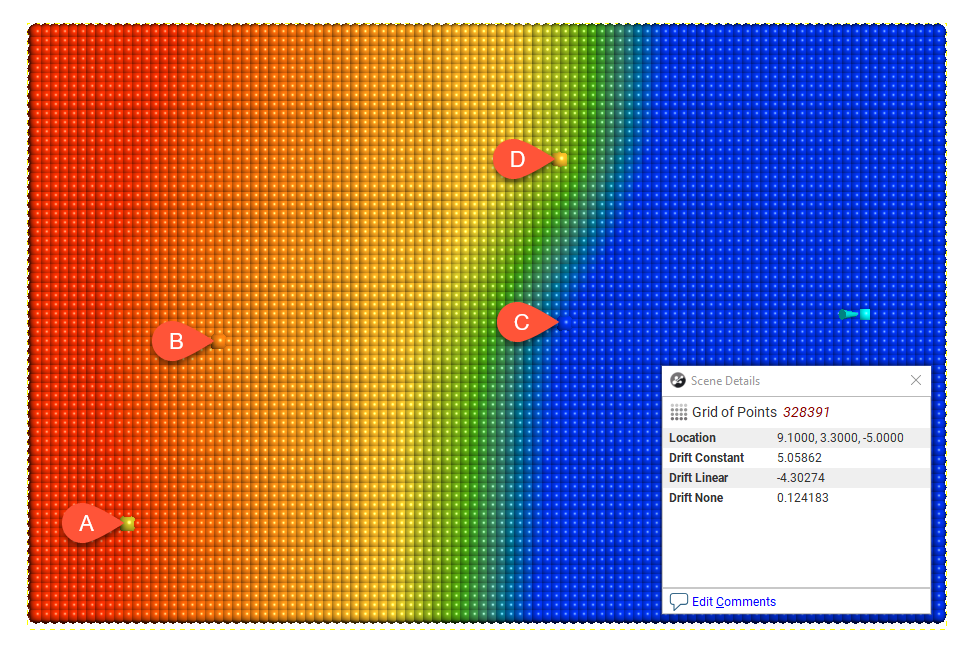
Drift = Linear
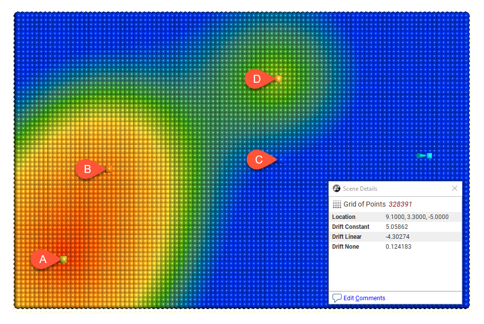
Drift = None
In this example, the boundary is larger than the extent of the data to illustrate the effect of different Drift settings.
Away from the data, the value of the interpolant when Drift is Constant and Linear is not reasonable in this case, given the distance from the data. The low value when Drift is None is more realistic, given the distance from the data.
If when using the spheroidal interpolant you get a grade shell that fills the model extents, it is likely that the mean value of the data is higher than the threshold chosen for the grade shell in question. If this occurs, try setting the Drift to None.
Accuracy
Leapfrog Geo estimates the Accuracy from the data values by taking a fraction of the smallest difference between measured data values. Although there is the temptation to set the Accuracy as low as possible, there is little point to specifying an Accuracy significantly smaller than the errors in the measured data. For example, if values are specified to two decimal places, setting the Accuracy to 0.001 is more than adequate. Smaller values will cause the interpolation to run more slowly and will degrade the interpolation result. For example, when recording to two decimals, the range 0.035 to 0.044 will be recorded as 0.04. There is little point in setting the accuracy to plus or minus 0.000001 when intrinsically values are only accurate to plus or minus 0.005.
The Linear Interpolant Function
Generally, estimates produced using the linear interpolant will strongly reflect values at nearby points and the linear interpolant is a useful general-purpose interpolant for sparsely and/or irregularly sampled data. It works well for lithology data, but is not appropriate for values with a distinct finite range of influence.
The linear interpolant function is multi-scale, and, therefore, is a good general purpose model. It works well for lithology data, which often has localised pockets of high-resolution data. It can be used to quickly visualise data trends and whether or not compositing or transforming values will be required. It is not appropriate for values with a distinct finite range of influence as it aggressively extrapolates out from the data. Most ore grade data is not well interpolated using a linear interpolant function.
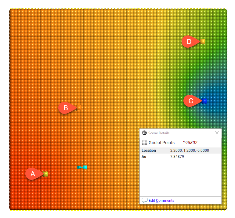
The linear interpolant function simply assumes that known values closer to the point you wish to estimate have a proportionally greater influence than points that are further away:
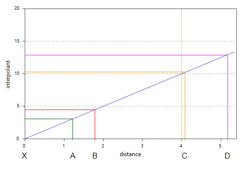
In the above diagram, points A and B will have the most effect on point X as they are closer to X than points C and D. Using the linear interpolant function in Leapfrog Geo gives a value of 7.85, which is between the nearby high grade values of A (10) and B (7). Because of their distance from X, the low grade values at C and D have a much weaker effect on the estimate of point X, and they have not dragged the estimate for X lower.
The parameters used to define a linear interpolant are Total Sill and Base Range, Nugget, Drift and Accuracy.
To edit the parameters for an interpolant, double-click on the interpolant in the project tree and click on the Interpolant tab. The graph on the tab shows how the interpolant function values vary with distance and is updated as you change interpolant parameters:
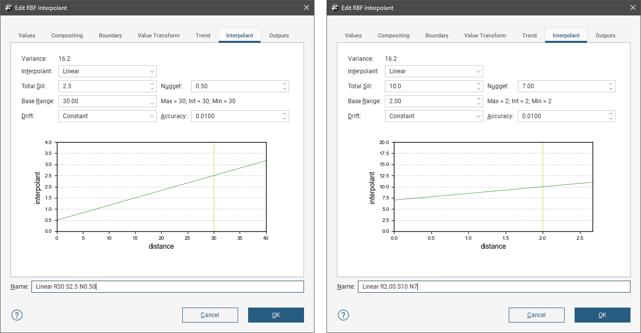
The yellow line indicates the Base Range. For this interpolant, the value of the interpolant is offset by the value of Nugget.
Total Sill and Base Range
A linear interpolant has no sill or range in the traditional sense. Instead, the Total Sill and Base Range set the slope of the interpolant. The Base Range is the distance at which the interpolant value is the Total Sill. The two parameters sill and range are used instead of a single gradient parameter to permit switching between linear and spheroidal interpolant functions without also manipulating these settings.
Nugget
The Nugget represents a local anomaly in values, one that is substantially different from what would be predicted at that point based on the surrounding data. Increasing the value of Nugget effectively places more emphasis on the average values of surrounding samples and less on the actual data point, and can be used to reduce noise caused by inaccurately measured samples.
Drift
The Drift is a model of the value distribution away from data. It determines the behaviour a long way from sampled data.
- Constant: The interpolant goes to the approximated declustered mean of the data.
- Linear: The interpolant behaves linearly away from data, which may result in negative values.
Here, the two Drift options for the interpolant are shown evaluated on grids:
Drift = Constant
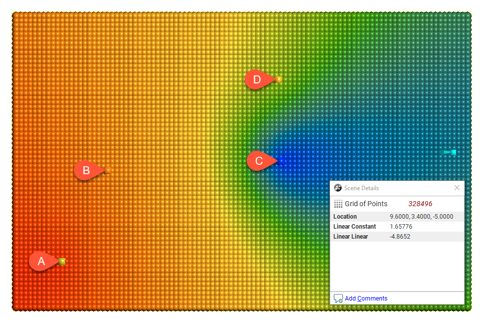
Drift = Linear
In this example, the boundary is larger than the extent of the data to illustrate the effect of different Drift settings.
Accuracy
Leapfrog Geo estimates the Accuracy from the data values by taking a fraction of the smallest difference between measured data values. Although there is the temptation to set the Accuracy as low as possible, there is little point to specifying an Accuracy significantly smaller than the errors in the measured data. For example, if values are specified to two decimal places, setting the Accuracy to 0.001 is more than adequate. Smaller values will cause the interpolation to run more slowly and will degrade the interpolation result. For example, when recording to two decimals, the range 0.035 to 0.044 will be recorded as 0.04. There is little point in asking Leapfrog Geo to match a value to plus or minus 0.000001 when intrinsically that value is only accurate to plus or minus 0.005.
Got a question? Visit the Seequent forums or Seequent support