Well Data
Well data forms the basis for creating models in Leapfrog Geothermal. Because well data often contains errors that reduce the reliability of a model, Leapfrog Geothermal has tools that help you to identify and correct errors and work with the data.
Well data defines the physical 3D shape of wells. It is made up of:
- A collar table, containing information on the location of the well.
- A survey table, containing information that describes the deviation of each well.
- At least one interval table, containing information on measurements such as lithology, date or any numeric or textual values. An interval table must also include collar IDs that correspond to those in the collar table and sample start and end depth.
A screens table can also be imported, if available.
When a project is first created, the only options available via the Well Data folder are for importing data. See Importing Well Data for more information on these options.
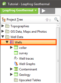
Once data has been added to the project, a Wells object will be created that serves as a container for the tables imported:
You can open each table by double-clicking on the table (![]() ). The table will be displayed and you can make changes. See Working with Data Tables. When there are errors in the data, the relevant table will be marked with a red X (
). The table will be displayed and you can make changes. See Working with Data Tables. When there are errors in the data, the relevant table will be marked with a red X (![]() ). See Correcting Data Errors in Leapfrog Geothermal for more information on fixing well data errors.
). See Correcting Data Errors in Leapfrog Geothermal for more information on fixing well data errors.
Leapfrog Geothermal also has tools for creating new lithology data columns from existing columns in order to solve problems with the well data. See Processing Well Data for more information.
To delete a lithology or numeric data table, right-click on the table in the project tree and select Delete. You will be asked to confirm your choice.
When you right-click on the well or collar table object in the project tree and select Delete, the resulting action will also remove all lithology and numeric data tables from the project. You will be asked to confirm your choice.
With Leapfrog Geothermal, you can also plan wells and evaluate them against any model in the project. See Planning Wells for more information.
The rest of this topic discusses options for displaying wells and viewing statistics on well data tables. It is divided into:
Displaying Wells
Viewing well data in the scene is an important part of refining well data and building a geological model. Therefore, Leapfrog Geothermal has a number of different tools for displaying well data that can help in making well data processing and modelling decisions. Display well data in the scene by dragging the Wells object into the scene. You can also drag individual tables into the scene.
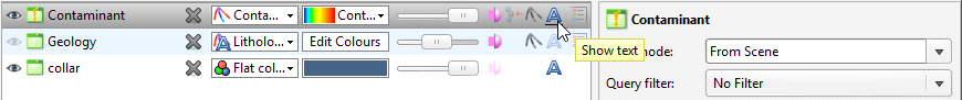
Once well data is visible in the scene, click on a well to view the data being displayed. You can also display the data associated with each interval by clicking on the Show text button (![]() ) in the shape list. Here, data display is enabled for two interval tables:
) in the shape list. Here, data display is enabled for two interval tables:
The Show trace lines button (![]() ) in the shape list displays all trace lines, even if there is no data defined for some intervals. The Filter trace lines option in the shape properties panel displays only trace lines for wells selected by a query filter. See the Query Filters topic for more information.
) in the shape list displays all trace lines, even if there is no data defined for some intervals. The Filter trace lines option in the shape properties panel displays only trace lines for wells selected by a query filter. See the Query Filters topic for more information.
Displaying Wells as Lines or Cylinders
You can display wells as lines or cylinders. You can also display the data associated with each segment. Here, the wells are displayed as flat lines:
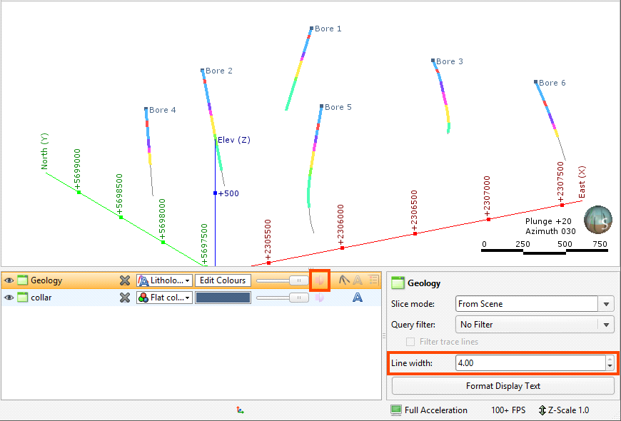
The width of the lines is set in the shape properties panel.
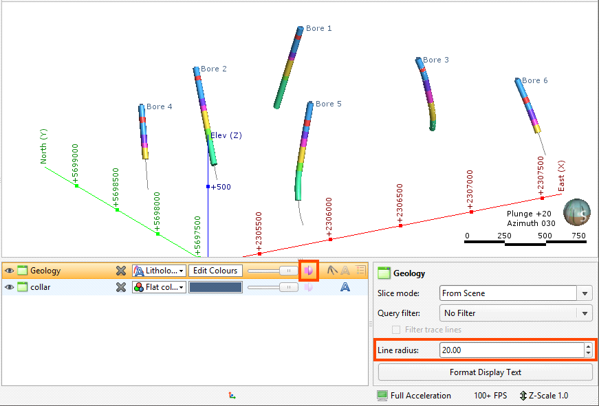
When the Make lines solid button (![]() ) is enabled, the well data is displayed as cylinders and the property that can be controlled is the Line radius:
) is enabled, the well data is displayed as cylinders and the property that can be controlled is the Line radius:
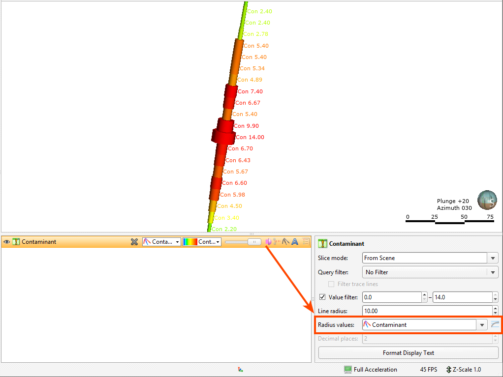
When numeric data is displayed, there is an additional option, to use a data column in the table for the cylinder radius:
When the log button (![]() ) is enabled, the log of values is used for the radius.
) is enabled, the log of values is used for the radius.
Hiding Lithologies
When lithology tables are displayed, you can hide some of the lithologies to help make better sense of the information in the scene. Click on the Edit Colours button in the shape list. In the window that appears, use the Show/Hide buttons (![]() ) to determine what segments are displayed:
) to determine what segments are displayed:
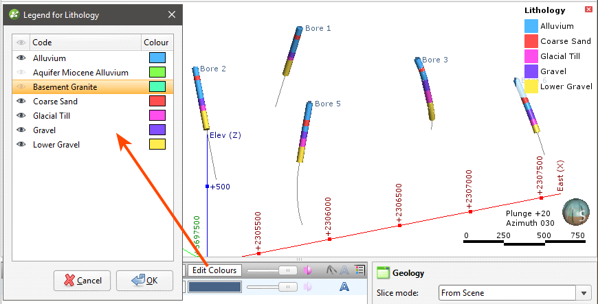
To select multiple lithologies, use the Shift or Ctrl keys while clicking. You can then change the visibility of all selected lithologies by clicking one of the visibility (![]() ) buttons.
) buttons.
Hiding lithologies in this way only changes how the data is displayed in the scene. Another way of limiting the data displayed is to use a query filter (see the Query Filters topic), which can later be used in selecting a subset of data for further processing.
Displaying a Legend
To display a legend in the scene, click the Show legend button (![]() ) for the table:
) for the table:
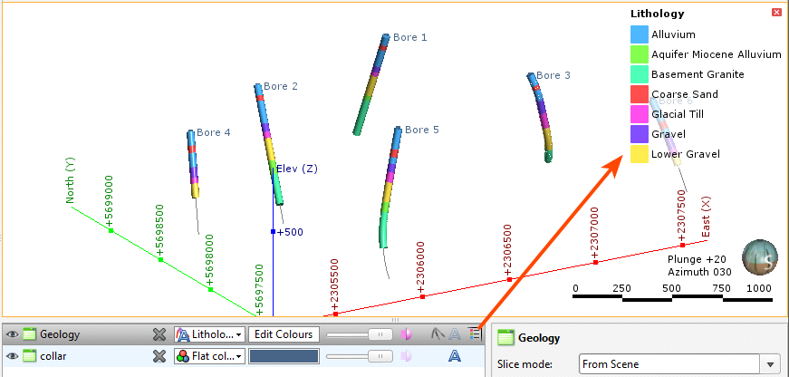
The legend in the scene will be updated to reflect lithologies that are hidden in the scene when you click Edit Colours and hide some lithologies.
Changing Colourmaps
To change the colours used to display lithologies, click on the Edit Colours button in the shape list. In the window that appears, click on the colour chip for each lithology and change it as described in Single Colour Display.
To set multiple lithologies to a single colour, use the Shift or Ctrl keys to select the colour chips you wish to change, then click on one of the colour chips. The colour changes you make will be made to all selected lithologies.
You can also import a colourmap, which is described in Colourmaps.
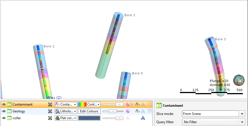
Viewing Multiple Interval Tables
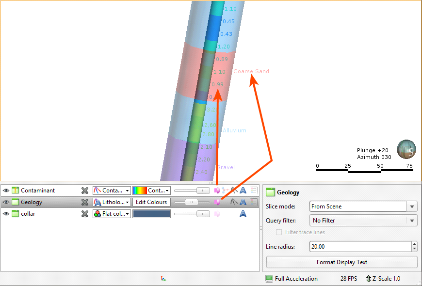
When viewing multiple interval tables, use the line and point size controls and the transparency settings to see all the data at once. For example, here, the geology table has been made transparent to show the contaminant intervals inside:
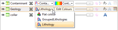
Selecting from Multiple Columns
When an interval table has more than one column of data, select the column to view from the view list:
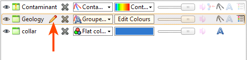
Some columns are editable, in which case you can click on the Edit button (![]() ) to start editing the table:
) to start editing the table:
Displaying Interval Data in the Scene
Wells can be displayed with the data associated with each segment. For example, in the scene below, contaminant values are displayed along the well:
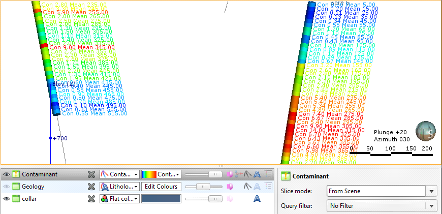
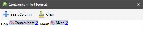
To view data in this way, select the table in the shape list, then click on the Format Text button. In the Text Format window, click Insert Column to choose from the columns available:
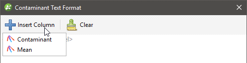
You can display multiple columns and add text:
Click OK to update the formatting in the scene. You can conceal the formatting in the scene by clicking on the Show text button (![]() ) in the shape list:
) in the shape list:
Clear text formatting by clicking on the Format Text button, then on Clear.
Displaying Well Graphs
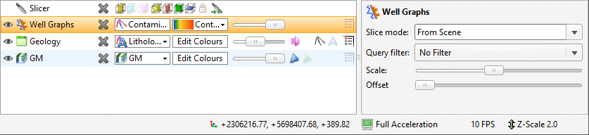
Downhole numeric data can be displayed in the scene as a bar graph and downhole points data can be displayed as a line graph. To display downhole data in this way, add the Well Graphs object to the scene. The Well Graph Style Manager will be displayed, showing the data columns available:
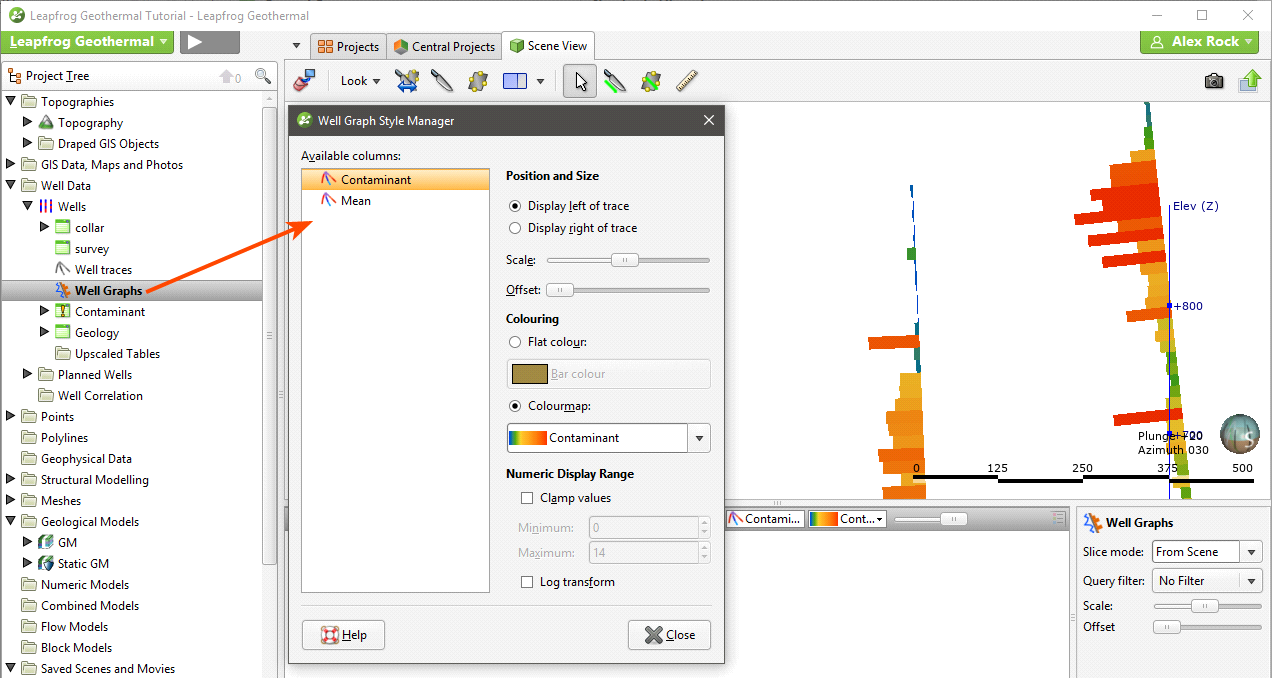
Data can be displayed to the right or the left of the well trace. Use the sliders to change the Scale and the Offset from the trace.
Data can be clamped, e.g. all values above the set maximum value will be set to the maximum value.
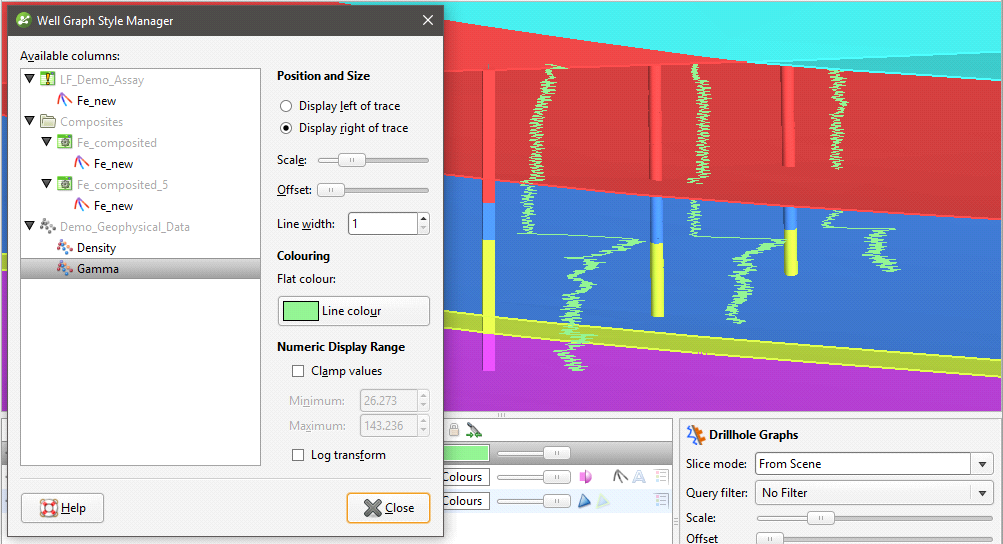
Downhole points can be displayed as a line, and you can change the Colouring, Scale and Offset of the line:
All changes made in the Well Graph Style Manager are automatically updated in the scene so you can experiment with the settings. Once you have closed the window, you can also change the Scale and Offset by clicking on the Well Graphs object in the shape list:
To select a different column to display, open the style manager by double-clicking on the Well Graphs object in the project tree or select a new column from the shape list.
If you are working in a new project into which you have just imported wells, the Well Graph Style Manager will open when you add it to the scene. If the Well Graph Style Manager does not open when you add the Well Graphs object to the scene, it is because the styles have already been set, perhaps by another user. You can change them by double-clicking on the Well Graphs object.
Viewing Well Data Table Statistics
To view statistics on an interval table, right-click on the table in the project tree and select Statistics. The following options are available:
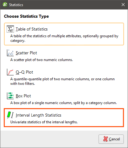
See the Analysing Data topic for more information on each option:
The Interval Length Statistics graph is a univariate graph, so for more information on the options available, see Univariate Graphs in the Analysing Data topic.
Right-click on a numeric column and select Statistics to open a univariate graph for that column.
Got a question? Visit the My Leapfrog forums at https://forum.leapfrog3d.com/c/open-forum or technical support at http://www.leapfrog3d.com/contact/support