
3D Array Plot
Use 3D Array Plot option, (geogxnet.dll(Geosoft.GX.IP.Plot3DArray;Run)*), to create a colour symbol plot in 3D space, analogous to an IP 2D pseudo-section.
Add 3D Array Plot to 3D dialog options
|
3D View name |
The name of the 3D View in which to plot the symbols. This 3D View may or may not exist; if it does not exist, it will be created. If the 3D View exists, any existing groups under the IP 3D Array node will be overwritten; note that you can always discard the changes. New groups will be added at the top of the existing ones in the tree. You are not prompted to specify a view name when the GX is run from within a 3D View (Add to 3D > IP > 3D Array Plot) – the array data will be plotted automatically in the current view. Script Parameter: IP_PLOT3DARRAY.MAP |
|
Plot point configuration |
The options offered depend on the current configuration. The current configuration is the default. The configurations with fewer electrodes than the current configuration will be provided as additional choices. See Application Notes below for more details. Select the plot point configuration as Dipole-Dipole, Pole-Dipole, or Pole-Pole. Script Parameter: IP_PLOT3DARRAY.PLOT_POINT_CONFIGURATION |
|
Plot coordinates |
This option appears only if your IP database contains both the local and georeferenced sets of coordinates. If both sets of coordinates are present, the default is to plot the points in the georeferenced coordinate system. However, you do have the option to plot in the local coordinate system as well. The Transmitter and Receiver tabs adjust to your selection. Script Parameter: IP_PLOT3DARRAY.PLOT_COORDINATES |
|
Transmitter 1 & 2 |
Transmitter 1 is required for all IP configurations. Define the coordinates of transmitter 1. Depending on the Plot point configuration option selected above, you may be prompted to enter the coordinates of Transmitter 2. You are prompted to provide the coordinates according to the Plot coordinates selection above. If plotting in the local coordinate system, you will be prompted to provide the channel along the survey line; this is the abscissa. Optionally, the coordinate normal to the survey line can also be provided. If plotting in the georeferenced coordinate system, you will be prompted to provide the georeferenced XY coordinates. The Z coordinate is optional. If left blank, it is assumed that the surface is a flat datum. Script Parameters: IP_PLOT3DARRAY. Tx1X, Tx1Y, Tx1Z IP_PLOT3DARRAY. Tx2X, Tx2Y, Tx2Z |
|
Receiver 1 & 2 |
Receiver 1 is required for all IP configurations. Define the coordinates of receiver 1. Depending on the Plot point configuration selected above, you may be prompted to enter the coordinates of Receiver 2. You are prompted to provide the coordinates according to the Plot coordinates selection above. If plotting in the local coordinate system, you will be prompted to provide the channel along the survey line; this is the abscissa. Optionally, the coordinate normal to the survey line can also be provided. If plotting in the georeferenced coordinate system, you will be prompted to provide the georeferenced XY coordinates. The Z coordinate is optional. If left blank, it is assumed that the surface is a flat datum. Script Parameters: Only available for the georeferenced coordinate system IP_PLOT3DARRAY. Rx1X, Rx1Y, Rx1Z IP_PLOT3DARRAY. Rx2X, Rx2Y, Rx2Z |
3D Symbols Tab |
|
|
Plot |
Define if All the selected data is to be plotted or if you will be windowing a rectangular Swath for display. The swath can be oriented in any azimuth direction and cut through the selected survey lines. The default is to plot all the selected data. See Application Notes below for more details. Script Parameter: IP_PLOT3DARRAY. PLOT_ALL_OR_SUBSET [1 – All selected data, 0 – defined swath] |
|
Plan map |
If you have selected the option All above, this parameter will not appear. If you have selected the option Swath above, you will be prompted to select an overlapping existing plan map on which to define the swath. Script Parameter: IP_PLOT3DARRAY.PLAN_MAP |
|
[Define] |
Clicking on this button will take you to the plan map, so that you define a rectangular swath. Click on the plan map to define the beginning of the central line of the swath, click again to define the end of the central line, and click a 3rd time to define the width of the swath. |
|
Electrodes |
By default, only plot points for which all contributing electrodes are located within the swath will be plotted (Tx & Rx). Sometimes, however, the second transmitter may be far away from the receivers but close enough for the data to have been configured as Dipole-Dipole. In this case, you would window the data by receiver locations only, regardless of the location of the transmitters (Rx only). You can also window the swath so that all plot points for which transmitters are in the swath (Tx only). Script Parameter: IP_PLOT3DARRAY.ELECTRODES_TO_PLOT [0 – Tx & Rx, 1 – Rx only, 2 – Tx only] |
|
Channel to plot |
Select the data channel to use for the symbol colour distribution. Script Parameter: IP_PLOT3DARRAY.CHAN |
|
Line selection |
Select the lines to display. The options are: the selected lines (the default option), the currently displayed line, and all the lines. Script Parameter: IP_PLOT3DARRAY. LINES [S – selected (default), D – displayed , A – all] |
|
QC channel |
Specify if data is to be masked. Masking can be done using the QC Resistivity and/or QC IP channels. Script Parameters: IP_PLOT3DARRAY.QC_IP [1 - QC IP is applied, 0 - QC IP is not applied] IP_PLOT3DARRAY.QC_RES [1 - QC RES is applied, 0 - QC RES is not applied] |
|
Show rejected points |
By default, the rejected readings are omitted from the plot. To show their location in grey, check this box. Script Parameter: IP_PLOT3DARRAY.PLOT_MASKED_VALUES_GREY [ 0 – Do not show rejected points (default), 1– display rejected points] |
|
Option |
The symbol is a sphere; its size can be specified as fixed or proportional to the Channel to plot values. Script Parameter: IP_PLOT3DARRAY.PROPORTIONAL [0 – fixed size, 1 – proportional] |
|
Symbol size |
The fixed symbol size. Press the calculator button to display the default estimated value. By default, the diameter is 1/4 of the a-spacing. Script Parameter: IP_PLOT3DARRAY.SYMBOL_SIZE |
|
Minimum |
The minimum symbol size. Required when plotting proportionally scaled symbols. Press the calculator button to display or reset the field to the default value calculated as the default Symbol size * 0.5. The sizes of the plotted symbols are scaled according to the data values in the Channel to plot. Script Parameter: IP_PLOT3DARRAY.SYMBOL_SIZE_MIN |
|
Maximum |
The maximum symbol size. Required when plotting proportionally scaled symbols. Press the calculator button to display or reset the field to the default value calculated as the default Symbol size * 1.5. The sizes of the plotted symbols are scaled according to the data values in the Channel to plot. Script Parameter: IP_PLOT3DARRAY.SYMBOL_SIZE_MAX |
|
Colour |
Select the colour scheme for colouring the symbols. If you hover the cursor over the colour scheme entry, a tool tip will display the name of the colour table. To modify the selection, click on the colour entry and then navigate through the scheme categories. If the colour scheme is a Zone file or an Index Transform File, the colour breaks will be placed at the values specified in the file and the Colour method remains disabled. Script Parameter: PLOT3DARRAY.COLOR |
|
Colour method |
Select one of the colour methods: As last displayed, Default, Histogram equalization, Normal distribution, Linear, or Log-linear. The As last displayed method will display each grid as it was displayed the last time the grid was viewed and the colour tables will be ignored. Script Parameter: IP_PLOT3DARRAY.COLOR_METHOD [0 - Default ; 1 – Linear; 2 – Normal distribution; 3 – Histogram equalization; 5 – Log-Linear; 6 – As last displayed] |
|
Reverse colour distribution |
Select Reverse colour distribution to reverse the distribution order of the selected colour scheme. Script Parameter: PLOT3DARRAY.REVERSE_COLOR [0 – default, 1 – reverse] |
|
Group hierarchy |
Select one of the grouping options available:
You will always have "Tx1 & Rx1", but depending on the configuration, you may or may not have a "Tx2 Rx2". Script Parameter: IP_PLOT3DARRAY.GROUP_HIERARCHY [0 – none, 1 – by line, 2 – by type] |
Topography Tab |
|
|
Grid |
Optionally, a topography grid can be displayed to the 3D view. Script Parameter: IP_PLOT3DARRAY.TOPO |
|
Colour |
Select the colour scheme for colouring the symbols. If you hover the cursor over the colour scheme entry, a tool tip will display the name of the colour table. To modify the selection, click on the colour entry and then navigate through the scheme categories. If the colour scheme is a Zone file or an Index Transform File, the colour breaks will be placed at the values specified in the file and the Colour method remains disabled. Script Parameter: PLOT3DARRAY.COLOR |
|
Colour method |
Select one of the colour methods: As last displayed, Default, Histogram equalization, Normal distribution, Linear, or Log-linear. The As last displayed method will display each grid as it was displayed the last time the grid was viewed and the colour tables will be ignored. Script Parameter: IP_PLOT3DARRAY.COLOR_METHOD [0 - Default ; 1 – Linear; 2 – Normal distribution; 3 – Histogram equalization; 5 – Log-Linear; 6 – As last displayed] |
Label Line ID Tab |
|
|
Plot line labels |
Select the Plot line labels to plot the line labels on the 3D View. Script Parameter: IP_PLOT3DARRAY.PLOT_LINE_LABELS |
|
Font |
Specify the fonts to use for the line labels in the 3D View. Script Parameter: IP_PLOT3DARRAY.FONT |
|
Size |
Specify the size of the fonts to use for the line labels in the 3D View. Script Parameter: IP_PLOT3DARRAY.FONT_SIZE |
|
Colour |
Specify the colour of the line labels in the 3D View. Script Parameter: IP_PLOT3DARRAY.FONT_COLOR |
Application Notes
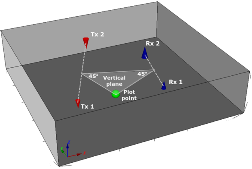
For each set of Transmitter-Receiver pairs, the symbol is placed at the 45° downwards intersection of the plane normal to the local topography. This plane passes through the midpoint of the line joining the transmitters and the line joining the receivers as illustrated below. While the horizontal scale is real, the vertical scale is not a real depth scale. This approach is analogous to the 2D pseudo-section display, where the vertical coordinate is used to visualize distinct readings with coincident horizontal locations.
The Wenner and Schlumberger array configurations do not lend themselves to a 3D array display because the midpoints of the transmitters and receivers are near coincident.
The symbols hang below the topography if one has been provided, however, the vertical location of the symbols should not be equated with real depths, and should not be directly compared with the vertical coordinate of any true 3D content such as geological features or resistivity voxels.
If the configuration does not contain a Transmitter 2 then the plane normal to the local topography passes through Transmitter 1.
If the configuration does not contain a Receiver 2 then the plane normal to the local topography passes through Receiver 1.
In the 3D view, each transmitter and receiver for each line are plotted as a separate group so that you be able to turn them on /off independently.
Plot Point Configuration
In essence, all IP surveys involve 4 electrodes; however, if the second transmitter and/or receiver is placed far enough from the survey area, it may be considered as located at infinity.
If the second transmitter is far away, the configuration is known as Pole-Dipole, and the coordinates of the second transmitter are generally omitted.
In the illustration below, the same IP data is shown in both Dipole-Dipole (left) and Pole-Dipole (right) configurations. The transmitter 2 electrodes are indicated on the left. On the illustration on the right, transmitter 2 is not taken into account, and as a result the 3D array plot is better aligned and easier to interpret.
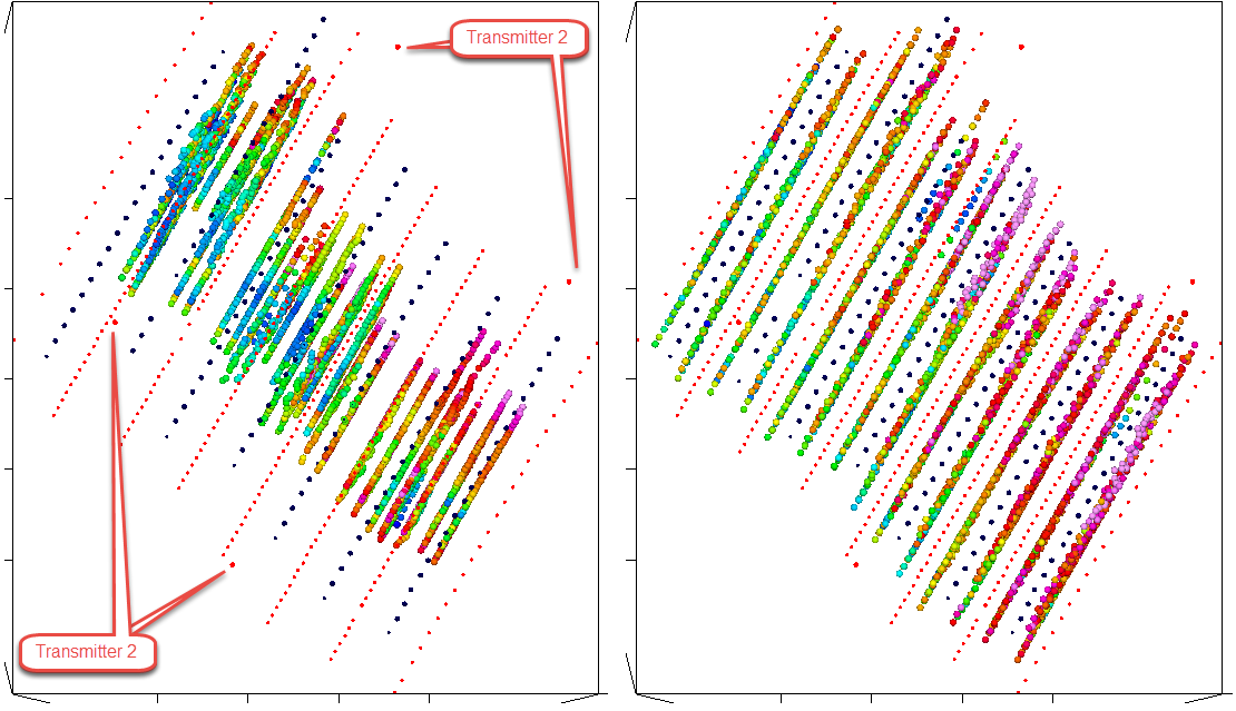
On the left the Dipole-Dipole configuration is selected. On the right the Pole-Dipole configuration is selected.
Defining the Swath
To view a narrow swath of the data that crosses multiple IP lines or to view a subset of data of a given line, you can define the swath on a plan map.
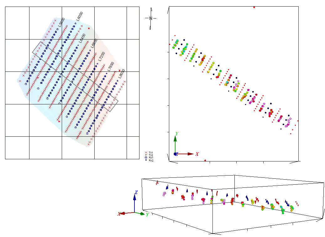
The swath is selected on the plan map (left). The resulting 3D Array plot of the swath is displayed on the right in 2 views.
Got a question? Visit the Seequent forums or Seequent support
© 2023 Seequent, The Bentley Subsurface Company
Privacy | Terms of Use