Quality Control by Null Coupling

Use the Quality Control > Null Coupling option, (geogxnet.dll(Geosoft.GX.IP.QCNullCoupling;Run)*), to reject rows whose Receiver pair resides on a Transmitter pair equipotential. This tool assumes a homogeneous subsurface.

Quality Control by Null Coupling dialog options

Line Selection	Select the lines to test. Script Parameter: IP_QC_NULLCOUPLING. LINES [S-selected(default), C-current, A- all]
Minimum Null coupling	The Null Coupling is a value between 0 and 1. Set the minimum coupling factor, below which the electrode geometry is assumed to be null coupled. All rows with a Coupling factor below this limit will be turned off. See Application Notes. Script Parameter: IP_QC_NULLCOUPLING. COUPLING_FACTOR [default=0.05]
Save coupling factor	It is recommended to save the coupling factor in the database. This tool assumes homogeneous subsurface when calculating the coupling factor . Nature however is far from being homogeneous. Depending on the variability of the resistivity of the area of interest, you may want to examine the coupling factor relative to your prior knowledge of the subsurface and relative location of the electrodes and occasionally override the automatic null calculation. Script Parameter: IP_QC_NULLCOUPLING. OUTPUT_COUPLING_FACTOR [Save-1(default), Not Save-0]
QC channel	The checked QC channels will be updated with the outcome of this QC test. Script Parameter: IP_QC_NULLCOUPLING. APPLY_TO_QC_IP [0 – unchecked, 1 – checked (default)] Script Parameter: IP_QC_NULLCOUPLING. APPLY_TO_QC_RES [0 – unchecked (default), 1 – checked]
QC selection	If Append existing is selected, the rows that are already turned off (QC value=DUMMY) will remain unaltered and the test will only be performed on rows that are still turned on (QC value=1). If Overwrite existing is selected, all previous QC channel settings will be reset to 1 prior to the test. Script Parameter: IP_QC_NULLCOUPLING. APPEND_MODE [0 – unchecked, 1 – checked (default)]
Transmitter 1 & 2	Define the coordinates of the 1st transmitter. This is required for all IP configurations. If the configuration supports a second transmitter, proceed to enter its coordinates. Script Parameter: IP_QC_NULLCOUPLING. T1X, T1Y, T1Z IP_QC_NULLCOUPLING. T2X, T2Y, T2Z
Receiver 1 & 2	Define the coordinates of the 1st and 2nd receiver. This is required for all IP configurations. Script Parameter: IP_QC_NULLCOUPLING. R1X, R1Y, R1Z IP_QC_NULLCOUPLING. R2X, R2Y, R2Z
Display null-coupled configurations	Check this box if you would like to display the null-coupled geometries on a plan map. It is recommended to use this option sparingly because if there is a large number of null coupled readings the map may become cluttered. If you would like to locate the null coupled readings one at a time, after running this tool, you could use the Show Contributing Electrodes tool. Script Parameter: IP_QC_NULLCOUPLING. PLOT_COORDINATES[ 0- don’t plot ( default), 1 – plot]
Map name	Select an existing map to show the null coupled geometries on. Script Parameter: IP_QC_NULLCOUPLING.MAP

Application Notes

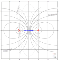
Given a good current flow between two transmitters placed on a homogeneous subsurface, the equipotentials will be distributed as indicated by the heavy grey lines in Figure 1. If two receiver electrodes are located on or near the same equipotential, there will be a negligible potential difference between them. Such a geometry is said to be "Null Coupled".

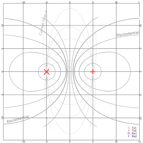
Given a good current flow in a homogeneous subsurface (thin grey lines) between 2 transmitters the equipotentials are distributed as indicated by the heavy grey lines.

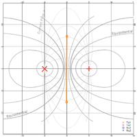
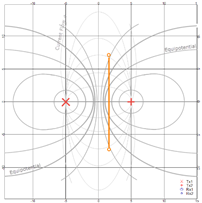
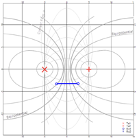
Null coupled geometries

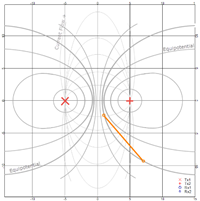
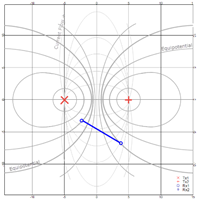
Well coupled geometries

The coupling factor for the homogeneous subsurface is approximated as follows:

1. Calculate the unit vector at the mid-point between the 2 receivers.
2. Calculate the unit-vector joining the mid-point of the receivers to the mid-point of the transmitters. For the Pole-Dipole configuration the unit-vector joining the mid-point of the receivers to the transmitter.
3. Calculate the magnitude of the dot-product of the above two vectors.
4. This dot product approaches 0.0 when the unit vectors are near parallel and 1.0 when they are normal.
5. The Null Coupling factor is saved in the database and used to test against the user specified minimum cutoff.

This tool applies to 3D geometries. In inline IP surveys the line joining the transmitters is parallel or near-parallel to the line joining the receivers which is analogous to a coupling of 1.0.

The above assumes a homogeneous subsurface. However this is rarely the case and the current distribution is rarely symmetrical about the transmitters. It is recommended to review the Null coupled rows within the context of the known geology.

As the receiver separation increases the above concept becomes less reliable because the deviation from homogeneity increases. However this approximation holds well for cases where the transmitter separation is much larger than the receiver separation.

Given the non-homogeneity of the subsurface, we recommend that you do not aim for the null couplings approaching zero, but rather start with a null coupling factor around 0.2 and adjust it further as needed.