
Crooked Section Grids
Vertically gridded profile data is frequently collected, extracted, or calculated along a line that has a non-straight path; such data is displayed in Oasis montaj using a specially defined grid orientation called "crooked section".
The following is an example of a crooked section grid displayed with a vertical exaggeration in a 3D View:
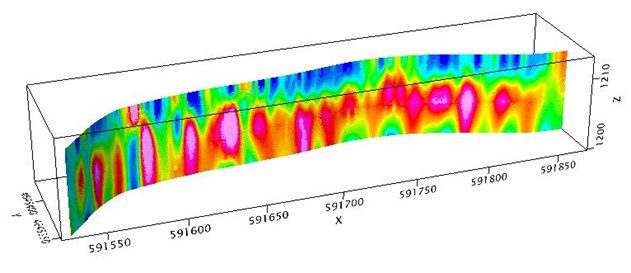
The data grid format used for the crooked section grids is the same as the one used for regular plan and section grids with the “Y” axis (grid columns) corresponding to the elevation and the “X” axis values corresponding to the distance measured along the line.
The information required to specify the grid “trace” is stored as an “orientation” inside the grid projection information (the IPJ class), and it consists of locations along the grid trace (line path) as well as the distance recorded at each location:
(x0, y0, d0), (x1, y1, d1), …. (xn-1, yn-1, zn-1)
The number of trace locations does not have to be equal to the number of columns in the grid, nor do the locations need to correspond exactly to the data locations; however, in many cases they do, and it is a good practice when defining a crooked section trace to ensure that the first and last points correspond to the first and last data column location in the grid.
Why is the distance along the line specified in addition to the locations?
In many cases, the distance is not simply the incremental straight-line distance between points. The distances correspond directly to the distances as defined in the grid “X” axis direction, and no assumptions are made about the exact path between each location (though for purposes of rendering in the third dimension, a straight-line join between points is assumed). This dependence on “D” instead of “X” and “Y” for grid positions means the path can be "thinned out" without losing the tie of each remaining location to an exact location in the grid.
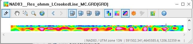
Rendering a Crooked Section Grid in the Grid View
The simplest view of a crooked section grid is in a grid window, where the grid is viewed “stretched out” with the “distance along the path” as the x-axis value and the elevation as the y-axis. The status bar still displays the correct location on the earth, because the cursor location is reprojected from the crooked section x-axis “distance” to the corresponding (X, Y) position for that distance.
Rendering a Crooked Section Grid into a Section View
To render a crooked section grid onto a section view, we project all the crooked section grid data perpendicularly onto the section. For instance, the section might be defined as the flat plane which intersects the crooked section at its beginning and at its end:
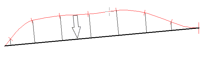
The effect of this projection is to compress the crooked section grid; moreover, the compression is not uniform – the parts of the section, which are angled the most with reference to the view, are compressed the most, while those parts closest to being parallel to the view are almost not at all compressed.
Mathematically, the crooked section (x, y) locations are rotated into the normal section's own coordinate system, where x is along the section, y is the elevation, and z is perpendicular to the section.
For each location Xs in the normal section, the two bracketing path locations are located: one with Xc lower than or equal to Xs, and one with Xc+1 higher than Xs. Using linear interpolation, the corresponding Dc and Dc+1 are used to determine the D corresponding to the required input location, and given the crooked section origin and grid DX value, the correct column (or columns) of data is determined to project to the required location in the normal section.
Rendering a Crooked Section Grid into a 3D View
To render a crooked section grid into a 3D View, the crooked section is first rendered (as above) onto the vertical plane that joins the beginning and end of the crooked section. Using the same transformation, the “Z” values in the progression – corresponding to the distance that the crooked section deviates from the plane are used to create a relief grid, that, when applied to the projected grid synthesizes the crooked section as if it were a coloured surface in 3D. The process creates two output grids, a “planar” grid and a “relief” grid. Both are rendered at the proper location on a defined plane in the 3D viewer, and as such do not have any type of section orientation. (You can see “planar” in the name of the AGG group of the Group Manager in the 3D viewer.)
Backtracks
Not all crooked section grids can be rendered in 3D using the above method. In addition, you cannot project a crooked section onto all possible flat sections. The reason is the "backtracking" in the projected section (the crooked section grids "double-back onto themselves"). Consider projecting the above “E-W” path onto an approximately “N-S” section:
Note that from locations 2 to 3, the projection reverses and overwrites existing values on the projection plane. Any projection needs to be 1-1, so in practice if this situation is encountered, the separation into a projected and relief grid is impossible. You will have the option to plot the grid as a “pixel plot”, where each grid cell is rendered as a single square in 3D. (This eliminates any smoothing effects.)
Got a question? Visit the Seequent forums or Seequent support
© 2023 Seequent, The Bentley Subsurface Company
Privacy | Terms of Use