Correlations

Use the Geochem Analysis > Correlations option (CHCORREL GX) to calculate the Pearson’s correlation between data channels and plot results in a correlation table on a map.

Correlation Plot dialog options

Data to analyze	"All ASSAY data" – all channels that are members of the ASSAY class will be analyzed. "Displayed ASSAY data" – only displayed channels that are member of the ASSAY class will be analyzed (this is the default setting). "All channels" – all numeric-type channels will be analyzed. "All displayed channels" – all displayed numeric-type channels will be analyzed. "Select ASSAY channels from list" -- select channels from a two-panel selection list.
Logarithmic option	The data being analyzed will be log-transformed before analysis depending on this option: "Default" – to use the LOG channel attribute to determine if the data should be log-transformed. "Logarithmic" – Log-transform all data. "Linear" – Do not log-transform any of the data.
Title	An optional title to be placed at the title box of the correlation plot. The default title is "Assay Correlations".
Colour code?	"Yes" to colour code the correlation values. The colours are determined by sample size and the significance level provided below. Colours are black, red, orange, green, cyan and grey respectively for very strong, strong, moderate, weak, very weak and null (not significant).
Significance level	Significance level of calculating correlation strength, it can be selected from 0.90, 0.95, 0.975 or 0.99 (usually 0.95).
Scatter plots in upper diagonal?	"Yes" to plot "mini" scatter plots in squares above the diagonal. Half the values are redundant, so no information is lost. The scatters are plotted without scales, and use the same log scaling as the correlation calculations. They are plotted to fit the squares, and will be plotted using the colour code.

Application Notes

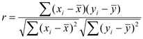
The correlations are calculated using Pearson’s correlation:

Colour coding:

Colours are determined by the sample size and the significance level described as follows.

Part of a correlation is spurious, originating by chance alone. This tends to increase with decreasing sample size. A measure of the spurious correlation is given by 

r (spurious) = square root ( (F/(N-2)) / (1.0 + F/(N-2)) )

where F is the spurious F value corresponding to a selected percentile, say 95%, of the probability distribution of the F statistic for a sample size of N. Consulting a table of F values, the degrees of freedom are 1 (column) and N-2 (row).

Let interval i = (1.0 - r(s)) / 5, a scale of correlation strength is given as

Calculated Sample Correlation Value Correlation Strength Colour

[r(s) + (4 x i)] to 1.0 very strong black

[r(s) + (3 x i)] to [r(s) + (4 x i)] strong red

[r(s) + (2 x i)] to [r(s) + (3 x i)] moderate orange

[r(s) + (1 x i)] to [r(s) + (2 x i)] weak green

r(s) to [r(s) + (1 x i)] very weak cyan

< r(s) null (not significant) grey

If the calculated sample correlation is larger than r(s) then it can be considered as significant at the level indicated.

If N is less than 2, then "(N<2)" is plotted instead of the correlation value.

A correlation matrix will appear as the selected group on the map. While the group is selected, you can move the mouse to a specific correlation of interest. If you then press the right mouse button, the groups "Maker" will appear as "Scatter tool…" at the bottom of the pop-up list. Select this option to display the scatter took for this data pair. Any number of scatter tools can be open at the same time, and all will be lined to each other and any open map displays of the survey area.