
Located Euler Deconvolution
Use the Euler 3D > Located Euler Decon menu option (E3XYEULER GX) to apply Euler depth deconvolution to obtain solutions (depths, etc.) from given X,Y locations in the current database.
Located Euler Deconvolution dialog options
|
Magnetic/Gravity grid |
Input Grid file name. Script Parameter: E3XYEULER.GRID |
|
X derivative grid |
Input X-Derivative Grid file name. Script Parameter: EULER3D.DX |
|
Y derivative grid |
Input Y-Derivative Grid file name. Script Parameter: EULER3D.DY |
|
Z derivative grid |
Input Z-Derivative Grid file name. Script Parameter: EULER3D.DZ |
|
Line containing grid peak locations |
The "group" line in the database in which the grid peak locations had been saved. Script Parameter: EULER3D.XYSOLGRP |
|
Line for Euler solutions |
The "group" line in the database to which the solutions (depths and indexes) are to be written. If the selected group already exists, it will be overwritten. If it left blank (the default), the solutions are written to the existent grid peak locations line. Script Parameter: EULER3D.SOLGRP |
|
Structural index |
Structural index, from 0.0 to 3.0 (default=1.0) See application notes below for details. Script Parameter: EULER3D.GI |
|
Max. % depth tolerance |
Maximum depth tolerance to allow (percentage) (default=15.0) All depth solutions with error estimate smaller than this tolerance will be accepted. The default is 15 percent. A smaller tolerance will result in fewer but more reliable solutions. Script Parameter: EULER3D.TOLRNC |
|
Max dist. to accept |
Maximum distance (from window center) acceptable (0 for infinite) (default=0.0). Solutions at a distance (from window center) greater than this maximum will not be accepted. Enter 0.0 for the default of infinity. This is the total distance in X, Y and Z, not just the horizontal distance. Script Parameter: EULER3D.MAXDIS |
|
Flying height |
Flying height of observation plane (default=0.0) For drape airborne surveys, enter the flying height. Depths will be reported as depth below ground by subtracting the flying height. By default, depth below plane of observation is reported. Script Parameter: EULER3D.OBSHGHT |
|
(or) Survey elevation |
Elevation of observation plane For barometric airborne surveys, enter the survey elevation. Depths will be reported as elevations by subtracting the model depth from the survey elevation. Note: By default the flying height will be used, unless a survey elevation is entered. Script Parameter: EULER3D.OBSELEV |
Application Notes
Located Euler Deconvolution
The Standard Euler deconvolution (E3DECON GX), moves a window of a fixed size over a grid of data and calculates Euler Deconvolution solutions for each window. There are typically many solutions, virtually one for every window location, which approaches the number of cells in the grid.
The Located Euler deconvolution (E3XYEULER GX) modifies this procedure by first locating only those windows which encompass peak-like structures in the data. A peak-finding routine is first run which locates peaks and estimates a window size using the locations of adjacent inflection points (the E3PEAKS GX). These locations and window sizes are then used to define the windows for Euler Deconvolution, using much the same algorithm as used in the E3DECON GX. The E3XYEULER GX typically produces far fewer solutions than the E3DECON GX because only a small subset of the grid cells will be the centers of "peaks" in the data.
Theory
The apparent depth to the magnetic source is derived from Euler’s homogeneity equation (Euler deconvolution). This process relates the magnetic field and its gradient components to the location of the source of an anomaly, with the degree of homogeneity expressed as a "structural index". The structural index (SI) is a measure of the fall-o ff rate of the field with distance from the source.
Euler’s homogeneity relationship for magnetic data can be written in the form:
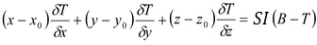
Where:
(x0, y0, z0) is the position of the magnetic source whose total field (T) is detected at (x, y, z,).
B is the regional magnetic field.
SI is the structural index, which is a measure of the fall-off rate of the magnetic field with distance from the source.
The Euler deconvolution process is applied at each solution. The method involves setting an appropriate SI value and using least-squares inversion to solve the equation for an optimum xo,yo,zo and B. As well, a square window size must be specified which consists of the number of cells in the gridded dataset to use in the inversion at each selected solution location. The window is centred on each of the solution locations. All points in the window are used to solve Euler’s equation for solution depth, inversely weighted by distance from the centre of the window. The window should be large enough to include each solution anomaly of interest in the total field magnetic grid, but ideally not large enough to include any adjacent anomalies.
Input and Output Channels
Structural Index (SI):
A structural index is an exponential factor corresponding to the rate at which the field falls off with distance, for a source of a given geometry.
From the following table choose an appropriate model for your structural index value:
SI
Magnetic Field
Gravity Field
0
Contact / Step
Sill / Dyke / Ribbon / Step
1
Sill / Dyke
Cylinder / Pipe
2
Cylinder / Pipe
Sphere
3
Sphere / Barrel / Ordnance
N /A
Another way to determine an appropriate structural index is to determine how many infinite, or reasonably large dimensions are present in a given model. The model SI is this number subtracted from the maximum SI for a given field, which is 3 for magnetic data and 2 for gravity data.
Note that a zero index implies that the field (magnetic or gravity) is constant regardless of distance from the source model. These solutions are physically impossible for real data, and a zero index represents a physical limit which can only be approached as the so-called ‘infinite’ dimensions of the real source increases. In practice, an index of 0.5 can often be used to obtain reasonable results when an index of zero would otherwise be indicated.
Geological Model
Number of Infinite dimensions
Magnetic SI
Gravity SI
Sphere
0
3
2
Pipe
1 (Z)
2
1
Horizontal cylinder
1 (X or Y)
2
1
Dyke
2 (Z and X or Y)
1
0
Sill
2 (X and Y)
1
0
Contact
3 (X, Y and Z)
0
NA
Got a question? Visit the Seequent forums or Seequent support
© 2023 Seequent, The Bentley Subsurface Company
Privacy | Terms of Use