
Bouguer Anomaly
Use the Gravity > Free Air, Bouguer Step by Step > Bouguer Anomaly menu option (geogxnet.dll(Geosoft.GX.Gravity.BouguerAnomaly;RunForGroundSurvey)*), or the Moving Platform Gravity > Bouguer Anomaly menu option (geogxnet.dll(Geosoft.GX.Gravity.BouguerAnomaly;RunForMovingPlatform)*), to carry out the following components of a gravity reduction:
(i) Bouguer anomaly calculation
(ii) Complete Bouguer anomaly (Bouguer anomaly + terrain correction)
Bouguer Anomaly dialog options
|
Database |
The name of the database is displayed for information. |
||||||||||||||
|
Survey type |
This entry is contextual and will appear if the tool is run from the Moving Platform Gravity menu. Specify the moving platform gravity survey type:
Script Parameter: GRBOUGUER.SURVEYTYPE |
||||||||||||||
|
Free air anomaly channel |
Select the input anomaly channel. For ground and airborne surveys, this is the gravity channel containing all the corrections including Free Air. In the case of shipborne surveys, the survey datum is relatively flat and at sea level, and a free air correction is not needed, so this channel could be the corrected gravity without a Free Air correction. For ground and airborne surveys, if there is a channel named "FreeAir" in the database, it will be selected. Script Parameter: GRAVRED.FREEAIR |
||||||||||||||
|
Terrain correction channel |
This is an optional entry. If previously calculated, select the terrain correction channel. By default, if there is a channel named "Terrain" in the database, it will be selected. Script Parameter: GRAVRED.TCORCH |
||||||||||||||
|
Terrain correction density
|
The default terrain density (in g/cm³) is set to the last terrain density used to calculate the terrain effect. You can, however, override this density if necessary. Should you opt to calculate multiple Complete Bouguer anomalies in a single run, for each density, the terrain effect channel data is rescaled using the provided correction density prior to be added to the output gravity channel. It is important to note that if the terrain effect is calculated near bodies of water, the density variability is not taken into account. In such instances, for each density, the terrain correction must be calculated separately. (See Complete Bouguer Anomaly below.) Script Parameter: GRTERAIN.DENST |
||||||||||||||
|
Elevation channel |
This is a contextual entry that appears for ground and shipborne surveys. Assuming you have made all the previous corrections (see Application Notes), this is the topography above the datum level. By default, if there is a channel named "Elevation" in the database, it will be selected. For shipborne surveys, this is the elevation of the instrument above Bathymetry (see Figure 2). Script Parameter: GRAVRED.ELEVATION |
||||||||||||||
|
DEM source |
This is a contextual entry that appears for airborne surveys. Specify the DEM source. If you do have the DEM as a channel in the database, select the Channel option. In the absence of a DEM channel, select the Grid option and specify below the DEM grid to sample into the database along the survey path. Script Parameter: GRBOUGUER.DEM_SOURCE (0: Channel, 1: Grid) |
||||||||||||||
|
Ground (DEM) elevation channel or DEM grid |
This entry depends on the DEM source selection:
|
||||||||||||||
|
Output Bouguer anomaly |
Specify the output Bouguer anomaly channel. Normally, this should be placed in channel "Bouguer". You have the option of changing the name in case you wish to create a number of Bouguer anomaly channels with different earth densities (see Number of Bouguer corrections below). Script Parameter: GRAVRED.BOUGUER |
||||||||||||||
|
Apply Bullard correction |
Check this box to apply the Earth curvature correction (see the Application Notes below). Script Parameter: GRAVRED.CURVATURE [1 – Yes (default), 0 – No] |
||||||||||||||
|
Latitude channel |
This is a contextual entry and will appear if the option Apply Bullard correction is checked. By default, if there is a channel named "Latitude" in the database, it will be selected. Script Parameter: GRAVRED.LATITUDE |
||||||||||||||
|
Number of Bouguer corrections |
Specify the number of Bouguer corrections. The default is 1. If a number > 1 is entered, you will be prompted to enter a Minimum earth density and a Maximum earth density. Incremental densities will then be calculated, and for each density, a Bouguer correction and Bouguer anomaly will be calculated. The density used for the calculation will be appended to the name of the output channels. To help you decide on the optimal density for the Bouguer correction, linear correlations for each density are calculated and reported in a popup window. See the Application Notes below for more details on the correlation coefficient. You can also display the Bouguer profiles for these channels in the database profile window to guide you on the Bouguer correction to use and the optimal density that can best remove the terrain effect. See the Application Notes below for more details on Bouguer anomaly calculation and Nettleton’s method[4]. Script Parameter: GRAVRED.CORRECTION_NUMBER |
||||||||||||||
|
Earth density |
Specify the density of the earth (in g/cm³) for calculating the Bouguer correction. Script Parameter: GRAVRED.DENSITY_EARTH |
||||||||||||||
|
Minimum Earth density |
Specify the minimum density of the earth (in g/cm³) for calculating the Bouguer correction. Available when the Number of Bouguer corrections is > 1. Script Parameter: GRAVRED.DENSITY_EARTH_MIN |
||||||||||||||
|
Maximum Earth density |
Specify the maximum density of the earth (in g/cm³) for calculating the Bouguer correction. Available when the Number of Bouguer corrections is > 1. Script Parameter: GRAVRED.DENSITY_EARTH_MAX |
||||||||||||||
|
[Other layer] |
Check this box if you wish to supply water/ice or overburden thickness and densities. Script Parameter: GRAVRED.OTHER_LAYER [1 – Yes (default) | 0 – No]
|
||||||||||||||
|
[More] Click to expand the section and view/modifiy the gravitational constant |
|||||||||||||||
|
Gravitational constant |
Over time, the gravitational constant changes ever so slightly. The default is set to the 2010 Gravitational constant in units of 10−11⋅m3⋅kg−1⋅s−2. See the Gravitational Constant section under Application Notes for further details.
Script Parameter: GRAVRED.GRAVITATIONAL_CONSTANT |
||||||||||||||
Application Notes
This GX assumes:
-
A gravity database is currently loaded (see Import Gravity Survey).
-
The tide, drift, latitude, and base station corrections have been applied (see Gravity Corrections).
1. Bouguer Anomaly
The free air correction only accounts for the difference in the elevation relative to the datum level. The topographical variation (presence of hills and valleys), however, affects the gravitational attraction. The Bouguer anomaly corrects the free air anomaly for the mass of (or lack of) rock that exists between the station elevation and the spheroid. In the case of airborne surveys, this is not the aircraft elevation but rather the DEM elevation above the datum level (Figure 1).
Furthermore, if the survey is conducted over water and/or ice, the Bouguer correction would take into account the water depth and the ice thickness. You are not prompted to provide the water and/or ice channel names. Instead, if the channels "Water" and/or "Ice" are present in the database, they are used in the Bouguer calculation. These two channels define the vertical distance (positive down) between the survey level and the topography (contact between rock and water) at the gravity station. Note that the "Water" channel contains the water depth at the gravity survey station location and that the ice thickness is included in the water depth. See Figure 2 below.
For shipborne surveys, if the datum coincides with the sea level (the Geoid), the water depth would be equivalent to the elevation and there would be no contribution to the Bouguer correction from the Earth' density below the datum. However, if the survey is conducted on a lake whose surface is different from the sea level (the Geoid), both the water and Earth densities contribute to the Bouguer correction component.
Bouguer Anomaly Correction Formula
For ground survey (including on lake surface) or shipborne (marine) survey:

For airborne survey:

Where:
Gb: Bouguer anomaly in milligals Gf: Free air anomaly D: Bouguer density of the earth in g/cm³ Hs: Station elevation in metres Dw: Bouguer density of water g/cm³ Hw: Water depth in metres (including ice) Di: Bouguer density of ice in g/cm³ Hi: Ice thickness in metres Gc: Curvature (Bullard B) correction Hg: Ground (DEM) elevation at survey station location in metres |
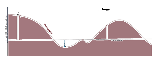
Figure 1: Schematic illustration of elevation channels and direction
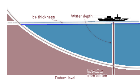
Figure 2: Schematic illustration of relation between elevation from Datum and water depth/ice thickness
Curvature Effect
The curvature correction (Bullard B) as a step in producing the Bouguer anomaly is to convert the geometry for the Bouguer correction from an infinite slab to a spherical cap whose thickness is the elevation of the station and whose radius (arc length) from the station is 166.735 km. Curvature correction depends on the station elevation (e.g. 1.1 mGal at 1000 m, 1.5 mGal at 2000 m, 1.2 mGal at 3000 m, 0.2 mGal at 4000 m, -1.5 at 5000 m and –3.9 at 6000 m), and latitude (ranging in dozens µGal). LaFehr’s (1991) formula is used for the curvature correction.
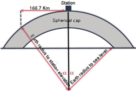
Figure 3: Schematic illustration (not to scale) of the spherical cap in Bullard B correction. The spherical cap surface radius of 166.7 Km , which is the outer radius or the Hayford-Boweie Zone O, is based on minimizing the difference between the effect of the cap and that of an infinite horizontal slab [LaFehr, 1991].
LaFehr expands the Bullard B correction calculation as:

Where:
BB: Bullard B correction γ: Gravitational constant ρ: Density h: Elevation (from sea level) R: Earth radius to the station: μ: Dimensionless coefficient: λ: Dimensionless coefficient: |


For context, below is what each of the Bullard corrections refer to:
- Bullard A: approximates the local topography (or bathymetry) by a slab of infinite lateral extent, constant density and thickness equal to the elevation of the point with respect to the mean sea level.
- Bullard B: curvature correction, which replaces the Bouguer slab by a spherical cap of the same thickness to a distance of 166.735 km.
- Bullard C: terrain correction, which consists of the effect of the surrounding topography above and below the elevation of the calculation point [Nowell, 1999].
2. Complete Bouguer Anomaly
The Complete Bouguer anomaly corrects the Bouguer anomaly for irregularities of the earth due to terrain in the vicinity of the observation point. The terrain correction GX’s can be used to calculate the terrain correction.

If multiple densities are desired:

Where:
Gcb: Complete Bouguer anomaly in milligals Gb: Bouguer anomaly in milligals (from [1]) Gt: Supplied terrain correction in milligals Di/Do: Ratio of the ith density over the density of the supplied terrain correction |
Linear Correlation Coefficient
If more than one Bouguer anomaly channel is requested, a Linear Correlation Coefficient is calculated for each density and reported in a popup window. Normally, to select the density that yields the least correlation between the shape of the topography and the calculated Complete Bouguer anomaly, you would visually focus on sections where the topography channel varies a lot (hills & valleys) then check if the gravity follows a similar trend and disregard the correlation in the remainder of the data. With this in mind, to use the Linear Correlation Coefficient as a decision aid, calculate it for such subsets of data. Select carefully a subset where you know that the topography is evident in the gravity data and apply the Bouguer correction for multiple densities. Once you find the best density (least correlation, coefficient closest to zero) use it to calculate the Bouguer anomaly for the entire dataset.
The Linear Correlation Coefficient equation is:
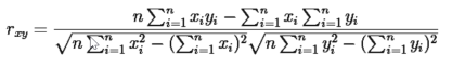
Where:
|
 : Complete Bouguer anomaly
 : Elevation
The correlation coefficient values reside between -1 and 1. A correlation coefficient closer to 1 indicates a close correlation between the x (Complete Bouguer anomaly) & y (elevation) profiles. A coefficient closer to -1 indicates an inverse correlation. As the coefficient approaches 0, the correlation decreases. The correlation that is the closest to 0 will be indicated with a star symbol (*) – as the least correlated one.
The correlation coefficients for the specified densities are reported at the end of the process. Furthermore, these coefficients are saved in the project working folder under the unique file name: BouguerNettletonCrossCorrelationCoefficientsyyymmdd.log
Nettleton’s Method
Nettleton’s method is based on the observation that the use of an appropriate reduction density will remove a correlation of observed gravity with topography. In this method, a gravity profile over a study area, in which there are significant sharp variations in elevation, is reduced by using a range of Bouguer reduction densities. The reduction density with a minimum correlation with elevation would give anomalies most representative of the underlying geologic structure.
The following assumptions must hold for Nettleton's method to apply:
- Nettleton's estimate fails if the topography is dominated by deeper geological structures.
- A relatively homogeneous density distribution in the area of interest.
- Sufficiently large (> 100 m) elevation differences and a uniform distribution of gravity measurements with respect to horizontal positions 'and elevations.
- A sufficient model of the regional field to be separated from the data.
Gravitational Constant
The gravitational constant (G) is a physical constant that is difficult to measure with high accuracy and which has varied broadly over time. G is re-evaluated every four years approximately. The table below lists published figures along with the uncertainty and source.
Published G values
Year |
G (10−11·m3⋅kg−1⋅s−2) |
Standard Uncertainty |
Reference |
| 1969 | 6.6732(31) | 460 ppm |
Taylor, B. N.; Parker, W. H.; Langenberg, D. N. (1 July 1969). "Determination of e/h, Using Macroscopic Quantum Phase Coherence in Superconductors: Implications for Quantum Electrodynamics and the Fundamental Physical Constants". Reviews of Modern Physics. American Physical Society (APS). 41 (3): 375–496. |
| 1973 | 6.6720(49) | 730 ppm | Cohen, E. Richard; Taylor, B. N. (1973). "The 1973 Least‐Squares Adjustment of the Fundamental Constants". Journal of Physical and Chemical Reference Data. AIP Publishing. 2 (4): 663–734. |
| 1986 | 6.67449(81) | 120 ppm | Cohen, E. Richard; Taylor, Barry N. (1 October 1987). "The 1986 adjustment of the fundamental physical constants". Reviews of Modern Physics. American Physical Society (APS). 59 (4): 1121–1148. |
| 1998 | 6.673(10) | 1500 ppm | Mohr, Peter J.; Taylor, Barry N. (2012). "CODATA recommended values of the fundamental physical constants: 1998". Reviews of Modern Physics. 72 (2): 351–495. |
| 2002 | 6.6742(10) | 150 ppm | Mohr, Peter J.; Taylor, Barry N. (2012). "CODATA recommended values of the fundamental physical constants: 2002". Reviews of Modern Physics. 77 (1): 1–107. |
| 2006 | 6.67428(67) | 100 ppm | Mohr, Peter J.; Taylor, Barry N.; Newell, David B. (2012). "CODATA recommended values of the fundamental physical constants: 2006". Journal of Physical and Chemical Reference Data. 37 (3): 1187–1284. |
| 2010 | 6.67384(80) | 120 ppm | Mohr, Peter J.; Taylor, Barry N.; Newell, David B. (2012). "CODATA Recommended Values of the Fundamental Physical Constants: 2010". Journal of Physical and Chemical Reference Data. 41 (4): 1527–1605. |
| 2014 | 6.67408(31) | 46 ppm | Mohr, Peter J.; Newell, David B.; Taylor, Barry N. (2016). "CODATA Recommended Values of the Fundamental Physical Constants: 2014". Journal of Physical and Chemical Reference Data. 45 (4): 1527–1605. |
| 2018 | 6.7430(15) | 22 ppm | Eite Tiesinga, Peter J. Mohr, David B. Newell, and Barry N. Taylor (2019), "The 2018 CODATA Recommended Values of the Fundamental Physical Constants" (Web Version 8.0). Database developed by J. Baker, M. Douma, and S. Kotochigova. National Institute of Standards and Technology, Gaithersburg, MD 20899. |
*The GX tool will search in the "...\Geosoft\Desktop Applications \gx" folder. The GX.Net tools, however, are embedded in the geogxnet.dll located in the "...\Geosoft\Desktop Applications \bin" folder. If running this GX interactively, bypassing the menu, first change the folder to point to the "bin" folder, then supply the GX.Net tool in the specified format.
References
- [1] T. R. LaFehr, "An exact solution for the gravity curvature (Bullard B) correction", Geophysics, vol. 56, no. 8 (1991), pp. 1179-1184. DOI: https://doi.org/10.1190/1.1443138.
- [2] T. R. LaFehr, "Gravity Corrections for Earth Curvature", SEG Technical Program Expanded Abstracts 1990, pp. 650-653.
- [3] D. H. Lee and T. D. Acharya, "Comparison of complete Bouguer anomalies from satellite marine gravity models with shipborne gravity data in East Sea, Korea", Journal of Marine Science and Technology, vol. 25, no. 6, pp. 625-632 (2017).
- [4] Rémy Villeneuve, "Nettleton's method applied to a field survey", redacted for the course Introduction to Geophysics, (University of Iceland, 2005).
Got a question? Visit the Seequent forums or Seequent support
© 2023 Seequent, The Bentley Subsurface Company
Privacy | Terms of Use