Create Regional Correction Grid

Use the Create Regional Correction Grid option (GRREGTER GX) to create a regional terrain correction grid for a survey.

The option is available with the Gravity and Terrain Correction extension under the following menus:

• Gravity >Terrain Corrections
• Moving Platform Gravity > Terrain Corrections

A regional terrain correction grid is calculated over a survey area based on a regional Digital Elevation Model (DEM) and at the resolution of a local, more detailed DEM. Note that the calculation of the regional correction grid is optional, and it is not required for the terrain correction. For surveys where additional data will be collected within the same survey area, calculation of the regional correction grid only needs to be determined once, thus reducing the overall time required for calculating the terrain correction each time it runs.

Create Regional Correction Grid dialog options

Regional DEM grid	This is the name of a regional DEM grid. This grid is normally compiled from government DEM data sets and extends significantly beyond the boundaries of a survey. It must cover the survey area in its entirety and extend well beyond. A typical grid cell size might be 250 m, and extend for 300 km beyond the Local DEM grid. Script Parameter: GRREGTER.REGDEMGRD
Local DEM (or water-depth / flight-elevation) grid	This is the most detailed local digital elevation model (DEM) grid available. This grid must cover the survey area and extend beyond by the Inner (local) correction distance. The regional terrain correction grid will have the same grid cell size as the Local DEM grid. If the local survey limits are not specified, the area of the local DEM grid is used. This grid is used to get a station elevation for terrain correction. For shipborne surveys the water depth grid should be provided here. This is the elevation relative to the datum (generally sea level) with the positive axis up. For airborne surveys the flight elevation grid should be provided here. Script Parameter: GRREGTER.LOCDEMGRD
Output terrain correction grid	This is the name of the output terrain corrected grid (see Application Notes). Script Parameter: GRREGTER.OUTGRD
Elevation units	The elevation units of the DEM grids (metres or feet). Script Parameter: GRREGTER.ELEVUNIT
Water reference elevation	Survey area water reference elevation in elevation units (default is 0.0). Script Parameter: GRREGTER.WATERELEV
Earth density	The density of the earth in g/cm³ (default is 2.67). Script Parameter: GRREGTER.DENST
Water density	The water density in g/cm³ (default is 1). Script Parameter: GRREGTER.WATERDENS
Outer (regional) correction distance	The distance to which to calculate a regional correction. This is normally significantly greater than the local correction distance but not larger than can be sampled from the regional DEM grid. By default, this distance will be the half the size of the regional grid. It is generally accepted that 300 km is a reasonable maximum. Script Parameter: GRREGTER.DOUTER
Inner (local) correction distance	This is the distance beyond which the regional correction will be calculated. This distance must match the local correction distance used in the Terrain Correction GX. The local correction distance will be rounded up to an integer multiple of the regional grid cell size. When running the Terrain Correction GX, the terrain correction inside this distance is calculated using the local terrain grid. Script Parameter: GRREGTER.DINNER
Optimization	For large regional grids, the terrain calculation can be quite slow. The optimization option accelerates the calculation by desampling the outer zones to a coarser grid (see Application Notes). Script Parameter: GRREGTER.OPT
Survey minimum X Survey minimum Y Survey maximum X Survey maximum Y	Specify a region that includes the limits of the survey. This is the region for which regional terrain corrections will be calculated. There is no need to calculate regional corrections over an area larger than the survey. Because the process of calculating the regional terrain effect can be slow, limiting the calculation to the area of interest can save time. If a region is not specified, the regional terrain grid will cover the area of the Local DEM grid. The [Scan XY] button can be used to scan the master database to determine the current limits of the database. Script Parameter: GRREGTER.MIN_X, .MIN_Y, .MAX_X, .MAX_Y
Survey type	The gravity survey types available are: Ground survey (including on lake surface) Shipborne survey (marine survey) Airborne survey Script Parameter: GRREGTER.SURVEYTYPE
[Scan XY]	Click this button to scan the current database and determine the limits over which a regional correction should be calculated. If more stations are to be added to the survey later, expand this region accordingly.

Application Notes

The calculation of the regional correction (beyond 1000 m) has been identified as the most computationally involved component of the calculation. The GRREGTER GX addresses this by calculating the regional terrain correction based on a coarse regional Digital Elevation Model (DEM) over a more finely sampled local DEM model that covers the survey area. This GX produces a "regional correction grid" that represents the terrain correction beyond the local correction distance reflected back on the local DEM grid coverage. The resulting output grid can be re-used to calculate detailed corrections at each observed gravity station.

The Terrain Correction GX will produce then full terrain corrections at each station by extracting an interpolated milligal value from the regional correction grid and adding it to the local correction calculated from a local, more highly sampled DEM grid. The local correction distance is the same as the one used to calculate the regional correction grid beyond that distance.

Optimization

The optimization option, on a test grid of dimensions 2500x2500 cells, improved the performance by a factor of 10 with only an accuracy loss of 3%. Optimization consists of using a 4x4 point Qspline interpolation of elevation data followed by desampling.

Regional and Local DEM Grids

Terrain correction requires a regional coarser DEM which would cover an area as much as 300 km beyond the survey area, and a more detailed local DEM. The local DEM should be sampled at a much finer cell increment and cover the survey area extended by the local correction radius. For example, a typical data set might have a regional DEM sampled at 250 metres with dimensions of 1200 x 1200 cells (300 x 300 km), and a local DEM sampled at 25 metres. The local DEM grid (flight elevation grid for the airborne survey) will be centered on the gravity survey area and extend at least by a local correction distance beyond the perimeter of the area.

Digital gridded terrain models are often available from government sources and can be used to simplify the application of regional terrain corrections. If there are enough known elevation points (X, Y, and Elevation), a gridded terrain model can be produced by using the Geosoft RANGRID or BIGRID programs.

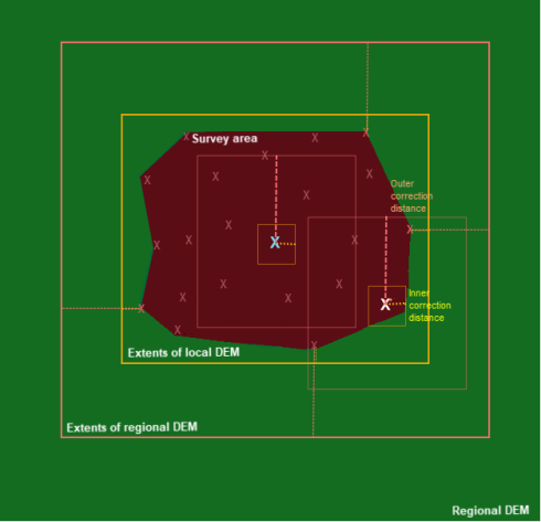
Figure 1: The Regional DEM grid (green) should cover at least the survey areas (filled brown polygon stations marked with Xs) extended by the outer correction distance (pink dashed lines). The pink rectangle denotes the required extents of the regional DEM grid. The yellow rectangle denotes the required extents of the local DEM grid.

Terrain Correction Methods

Terrain corrections are calculated using a combination of the methods described by Nagy [1966] and Kane [1962].

To calculate the correction at each gravity station, the DEM grid is resampled and centered on the station. The correction is calculated based on a near zone (1 cell radius ring from the station), intermediate zone (2 to 16 cells radius ring) and a far zone (beyond 16 cells).

For ground surveys, in the near zone, the algorithm sums the effects of four sloping triangular sections, which describe a surface between the gravity station and the elevation at each diagonal corner. In the intermediate zone, the terrain effect is calculated for each point using the flat-topped square prism approach of Nagy. In the far zone, (greater than 16 cells), the terrain effect is derived based on the annular ring segment approximation to a square prism as described by Kane.

For shipborne/airborne surveys, corrections are calculated using the flat-topped square prism approach of Nagy for the near and intermediate zone and using the rod formula [Telford et al.,1976] for the far zone.

For more processing efficiency, the far zone calculation can be optimized by desampling the outer zone to a coarser averaged grid (i.e., by enlarging the size of each segment to 2x2 cells for 16 to 32 cells radius, to 4x4 cells for 33 to 64 cells radius, and so on). The calculation is carried from the inner (local) correction distance up to the specified outer (regional) correction distance.

Special considerations and assumptions:

• The DEM grid is reflected on its edges in order to always provide corrections out to the required radius.
• Dummy terrain values are interpolated using a weighted average of the surround points.
• The system uses the grid average elevation to compensate for terrain effects in the area past the outer (regional) correction distance.
• Gravity stations are assumed to lie on a surface defined by the DEM (or on the ship for the shipborne survey case and on the airplane for the airborne survey case). If the position of the gravity stations deviates significantly from this surface, the regional component of the terrain correction will not be correct.

The output terrain correction grid is calculated for a ground density of 1.0. When used in the Terrain Correction GX, it is scaled by the provided earth density, and over water it is scaled by the ratio of the water density over the earth density (water_density/earth_density).

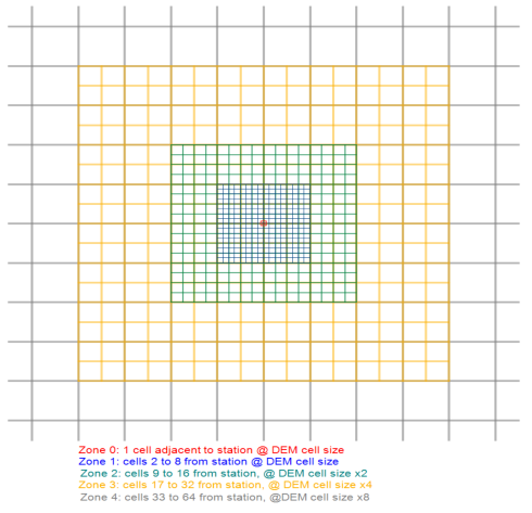
Figure 2: The illustration shows the first five zones

The process consists of the following steps:

1. Regional DEM is windowed to a bounding rectangle of the survey area + outer distance (shown with the orange rectangle).
2. Regional DEM is re-gridded to the cell size of the local DEM grid (CS_L ) so that it coincides with the Local DEM grid (Figure 2).

3. For each gravity station, the surrounding area is divided into zones. The number of zones depends on the cell size and the outer distance and are determined as follows:
   Number_of_Cells: N = DIST_Ou / CS_L
   Shifting our thinking centered on a given gravity station (Figure 2):

• The four cells around each gravity station are treated as Zone 0 and as slopped prisms.
• Cells 2:8 all around each gravity station will be used at cell size CS_L and constitute Zone 1.
• Cells 9:16 around each gravity station will be used at cell size 2x CS_L and constitute Zone 2.
• Cells 17:32 around each gravity station will be used at cell size 4x CS_L and belong to Zone 3.
• Cells 33:64 around each gravity station will be used at cell size 8x CS_L and belong to Zone 4.
• Cells 65:128 around each gravity station will be used at cell size 16x CS_L and belong to Zone 5.

This process continues until either Zone < 14 or cells around gravity station < half grid size.

4. Both the local and regional grids are dessampled number_or_zone times at cells 1x  2x  4x  etc...
5. At each gravity station, the terrain effect is calculated as the sum of the effect of all prisms within a circle of outer radius centered on the gravity station (indicated as orange circles above).
• The four prisms in Zone 0 are treated as triangular base prisms with a sloping top.
• The height of each prism in zones >=1 is relative to the gravity station for which the effect is calculated; that is the difference between the current gravity station elevation and the DEM. This height is positive for hills above the station elevation and negative for valleys below the datum of the station. The cross section of each prism depends on its distance from the gravity station as indicated below.

References

- D. Nagy, "The Gravitational attraction of a right rectangular prism", Geophysics, vol. 31, no. 2 (1966), pp. 362–371.
- M. F. Kane, "A Comprehensive system of terrain corrections using a digital computer", Geophysics, vol. 27, no. 4 (1962), pp. 455-462.
- W. M. Telford et al., Applied Geophysics, (Cambridge: Cambridge University Press, 1976), p. 59.
See Also:
Got a question? Visit the Seequent forums or Seequent support
© 2023 Seequent, The Bentley Subsurface Company
Privacy | Terms of Use