
Inverse Distance Weighted Gridding
Use the Inverse Distance Weighted Gridding method to create a grid from point data using an Inverse Distance Weighting algorithm. The method is used primarily to interpolate geochemistry data. Use the geogxnet.dll(Geosoft.GX.GridUtils.IDWGridding;Run)* to create a grid file from a channel in a database.
Inverse Distance Weighted Gridding dialog options
 button to calculate the default cell size. See the Application Notes below for details on calculating the default cell size.
Application Notes:
Default Grid Cell Size
The grid cell size (the distance between grid points in the X and Y directions) should normally be ¼ to ½ of the line separation or the nominal data sample interval. If not specified, the data points are assumed to be evenly distributed, and the area rectangular. The default cell size is then defined by the following formula:

Where:

Anti-aliasing
Prior to gridding (and after any log or log-linear transformation), data is pre-processed using an anti-aliasing technique. All values falling inside any single grid cell are averaged, and the data is then represented by the single averaged value at the grid cell centre. Any error in the spatial representation of features introduced by this step will never exceed one-quarter of the Nyquist wavelength, which is equal to 2 cell sizes.
Definition of the Weighting Slope and Power
The inverse distance weighting is a deterministic method for multivariate interpolation using a known set of data values at known locations. The grid values at each x,y point are calculated using a weighted average of the known data values within the defined search radius. The weight attributed to each known data value is inversely proportional to its distance from the grid x,y point. Applying a power to the weights will modulate the influence of each known data value as a function of distance. Furthermore adding a slope factor moderates the sharpness of the weights and prevents them from reaching a large dynamic range in close proximity to the x,y point. The weight of each of the n points within the search radius centered on a point x,y, is defined by the equation:
These weights must be normalized. The normalized weight equation becomes:
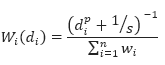
Where:
di is the distance of each of the n known data values gi within the search radius from the grid point x,y
n is the total number of gi values within the search radius
p is a constant power
s is a constant slope
At each grid cell x,y, the value will be calculated as:
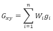
Where:
Gxy is the output grid value at location x,y
gi is the input data values within the search radius
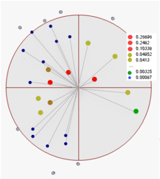
Figure 1: The normalized weights (legend) of all gi data points (indicated within the search radius) are calculated. Points outside the search radius are ignored. Then, equation Gxy=∑ni=1Wi gi is applied.
Using a default power of 2 and a slope of 1, produces a standard Gaussian bell-shaped weighting function. A slope > 0 ensures that the weight remains finite at zero distance. Decreasing the slope tends to flatten the bell, resulting in greater weighting of points away from the grid cell, and hence greater smoothing.
A power < 2, or a slope <1, may result in over-smoothing the data.
The following table shows the effect of various slopes on the weighting given at various distances away from the centre cell. The weights have been normalized so the weight at the cell centre is equal to 1
|
|
weighting of centre cell |
weighting 1 cell away |
weighting 2 cells away |
weighting 3 cells away |
weighting 4 cells away |
|---|---|---|---|---|---|
|
P = 2, S = 0.2 |
1 |
0.83 |
0.55 |
0.36 |
0.24 |
|
P = 2, S = 0.5 |
1 |
0.67 |
0.33 |
0.18 |
0.11 |
|
P = 2, S = 1 |
1 |
0.5 |
0.2 |
0.1 |
0.056 |
|
P = 2, S = 2 |
1 |
0.33 |
0.11 |
0.053 |
0.03 |
Clearly, as the slope increases, the weighting is more tightly concentrated about the centre cell. The search radius should also be chosen based on the fall-off of the weighting function. Increasing the search radius beyond where the weighting function is significant, will have little effect on the results, and may result in large increases in processing time, since the processing time varies in proportion to the cube of the search radius. (Remember that the search radius is specified in ground units, not as a multiple of cell sizes.)
The yellow asterisk icon ( ) displayed in front of a parameter name indicates that this parameter is required.
Got a question? Visit the Seequent forums or Seequent support
© 2023 Seequent, The Bentley Subsurface Company
Privacy | Terms of Use