
Add Geosurface to 3D View
In the 3D Viewer, use the Add to 3D > Geosurface menu option to add a geosurface to the current 3D View.
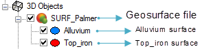
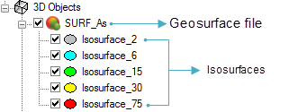
After the geosurface has been added to the 3D Viewer, the 3D Objects tree list will show the geosurface file name as the top level and below that, the surfaces within the geosurface.
Example 1: Geosurface created as output from wireframing:
Example 2: Geosurface containing isosurfaces:
With a geosurface file or a surface layer selected in the tree list, the Attributes tab will give additional information about the source file used to create the geosurface, whether the surface is open or closed, and the total surface area or total volume.
With a surface selected in the tree, from the Attributes tab, the rendering can be set to: Smooth, Fill or Edges.
Changing the colour for a surface will update the icon's colour in the 3D Objects tree as well as the colour of the surface in the 3D model.
Application Notes
The total volume for closed surfaces created through wireframing is calculated using the divergence theorem, also known as Gauss’s theorem. Because there are numerous intermediate calculations for every triangle on the surface, there may be rounding effects due to the internal constraints of the number of representations in the CPU. This can add up for surfaces with many triangles and/or where the XY extents are much larger than the extents for Z (e.g., in UTM coordinates).
During the calculation, a computational method called interval arithmetic is used that determines an upper and lower bound on the volume computed. This essentially adds up the estimates of individual errors as they are accrued for every triangle.
Got a question? Visit the Seequent forums or Seequent support
© 2023 Seequent, The Bentley Subsurface Company
Privacy | Terms of Use