The Variogram

The variogram of the data (in fact, this is the semi-variogram, but we call it the variogram for brevity) is calculated using the expression:

This function shows the correlation of observed data as a function of distance between points.

The variogram shows the anticipated increase in variability as h increases. At the right end of the variogram, the variability may appear to decrease in many cases (somewhat so in the example above), but this is usually the result of too few pairs of samples for the statistics to be valid. Kriging (KRIGRID) requires a model of the observed variogram to determine the weighting factors used in the kriging matrix. Although observed variograms can appear quite noisy, it is important that the model used is both smooth and has increasing variability with increasing h. KRIGRID offers a number of standard models which you can use to best approximate the observed variogram. The statistical accuracy of kriged results is related to how close the model is to the observed variogram. KRIGRID will write out the variogram of the data in the ASCII text file specified by the -vo= command line parameter.

The file is a standard Geosoft data file that begins with comment lines containing information about the variogram model, in this case a power model with a power of 1 (linear). The model parameters are listed (model, nugget, slope and power), together with SIGMA, which is the RMS difference between the variogram model and the observed variogram. The data columns contain the distance between samples (VH), the observed variogram (VG), the modelled variogram (VM), the number of points averaged to calculate the variogram (NP), and an index (I).

Using Variogram Models

Kriging (KRIGRID) supports a number of standard models in addition to a user-defined model, all of which are described below. If you run KRIGRID without regard for the model, the linear model will be used by default.

Power Model

The linear power model (n = 1) is the default model used in kriging (KRIGRID). Only the power model can be determined automatically by KRIGRID - all other models require you to enter the model parameters. KRIGRID uses least square fitting to determine the slope of the linear model for a line that starts at (0,0). If this is unacceptable, use the control file parameter "nugget" to set the intercept, and the parameter "range" to define the slope.

The power model follows the expression:

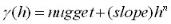
As a guideline, the power (or linear) model can be acceptable when the nominal group of nearest and second-nearest data points are well within the area of the model where the model line is still close to the observed variogram. This is seldom the case for clustered data.

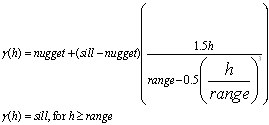
Spherical Model

The spherical model is the most common used in geological situations. To use the spherical model, you must first plot out the variogram of the data you are working with and determine the optimum range, nugget and sill.

The spherical model has the following expression:

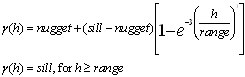
Gaussian Model

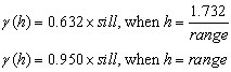
To use the Gaussian model, you must first plot out the variogram of the data you are working with and determine the optimum range, nugget and sill. With this model, the sill is actually never reached and at the range of the model is 5% less than the sill.

The Gaussian model has the following expression:

Where:

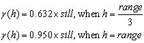
Exponential Model

To use the exponential model, you must first plot out the variogram of the data you are working with and determine the optimum range, nugget, and sill. As with the Gaussian model, the sill is actually never reached. At the range, the model is 5% less than the sill.

The exponential model follows the expression:

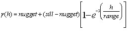
Where: