IP Settings

Within the VOXI document, use IP > IP Settings to modify inversion settings.

IP Settings dialog options

Error statistics	By default, L1 statistics method is applied to least squares fitting. Use this method if the data contains extreme outliers. L1 simulation is done by down-weighting the leverage data points with a large misfit. Apply the L2 statistics method to the least squares fitting if the data does not have extreme outliers. L2 simulation does not apply down-weighting.
Number of times	Specify the number of times the down-weighting is applied. 5 times is recommended. Beyond that, the inversion switches back to standard L2 statistics.
Numerical method	The two standard approaches for solving DCIP partial differential equations (PDE) are the Finite element method and the Finite volume method. Each method has advantages and disadvantages (see Application notes).
Winnow	The decimation applied to IP/Resistivity inversion differs from that of the other geophysical methods, in that rather than being based on a geographical reference, the measured data is winnowed based on its degree of impact on the inversion process, Generally winnowed data behaves better along the convergence path. By default this box is not checked and no winnowing is applied.
Samples per box	Define the number of measurements to retain in each sub-domain (box). If winnowing is applied the default number of samples per sub-domain is set to 1.
Box dimensions	Define the dimensions of the sub-domain. The sub-domain is defined in terms of number of voxel cells (see Application Notes). The winnowing process identifies the measurements that affect each sub-domain, ranks them in order of their impact on the inversion process, and pass only the first “Samples per box” measurements to the inversion. The default is X,Y,Z=1,1,1

Application Notes

Statistics

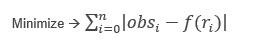
The L1 or L1-norm is the sum of the Least absolute differences of the observed obs_i and predicted values f(x_i) at the observation points r_{i (i=0,1,2…n)} The inversion attempts to minimize this sum.

The L2 or L2-norm is the sum of the squares of the Least differences.

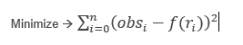
The DC IP data often contains extreme outliers. It is generally desirable to reduce the influence of these outliers. The L2 statistics are biased by extreme values which may result in a dominating influence on the fit whereas L1 statistics down-weigh this influence. The L1 simulation is almost analogous to the traditional “Iterative Reweighted Least Squares Method” (see Iterative Reweighted Least Squares).

Numerical Method

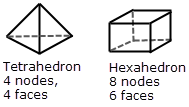
The finite volume (FV) mesh consists of hexahedra volumes, while the finite element (FE) mesh is a tetrahedral adaptive mesh. It is important to note that the OM 3D viewers cannot currently display a tetrahedral mesh. The FE mesh is adapted on the knowledge that the potential decays as r^-1 away from a current source. The inversion parameterization is always a rectangular mesh, as defined by VOXI. For FV forward modelling the forward model mesh and the inversion parameterization are the same. For the FE forward modelling, the FE mesh is also adapted to the rectangular inversion mesh in such a way that a particular group of tetrahedra define exactly the volume of an inversion parameter. A hexahedron can be subdivided into 5 tetrahedra. This allows exact conversion between the inversion parameterization mesh and the FE forward modelling mesh.

Winnowing

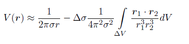
The measured data is decimated using the simple notion of dropping data which exerts little impact on the inversion process. To illustrate the approach let’s consider a uniform halfspace earth with conductivity σ and a small conductivity perturbation σ+Δσ in the sub-volume ΔV.

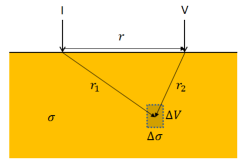
Figure 1: A uniform half space model with small conductivity perturbation.

The potential V(r) can be expressed as:

The sensitivity of a measurement in the sub-domain ΔV to the change in the conductivity is:

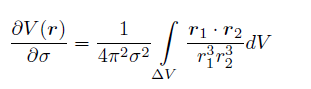
Which is indicative of the effect that each measurement exerts on a voxel volume ΔV. For each current electrode(s), the larger the distance of the potential electrode(s) from the sub-domain, the smaller it’s impact.

In the schematic illustration of Figure 1.2 the current is injected at electrode I and the resulting potential is measured at the potential electrodes V₁ through V₇. For simplicity the Y coordinate is omitted.

If the voxel model is subdivided into sub-domain boxes of dimensions X,Z=6,4, as indicated by the dashed lines, the most impactful measurements in box 1 in order of importance are V₁ then V₂.. In box 2 V₄ then V₃, and in box 3, V₆ then V₅.

In this case a winnowing process that retains 1 measurement in each 6x4 sub-domain will winnow V₂, V₃, V₅ and pass V₁, V₄, V₆, V₇ to the inversion process.

This process is repeated for every current location and easily generalized to more complicated electrode distributions.

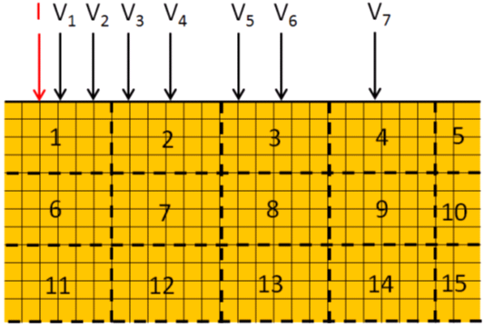
Figure 2: A voxel model subdivided into boxes under a pole-pole survey.

The percentage of the retained measurements sent to the inversion is reported in the log file under Important data. Furthermore the number of retained measurements and the number of winnowed measurements are also reported in the log file under Parameters.

References

-
Finite Volume: Finite Volume Metho2023IP Settingsds, Randal J. LeVeque, 2002, Cambridge Press.
Finite Element: Finite Elements for Electrical Engineers, Peter P. Silvester, Ronald L. Ferrar, 1966, Cambridge Press.
Finite Difference, Finite Element and Finite Volume Methods for Partial Differential Equations, Peiro J. Sherwin S., 2005, Department of Aeronautics, Imperial College, London, UK
Got a question? Visit the Seequent forums or Seequent support
© 2024 Seequent, The Bentley Subsurface Company
Privacy | Terms of Use