
Geophysical Data
The types of geophysical data that can be imported into Leapfrog Works are:
- 2D Geophysical Points
- 2D Grids
- 3D Grids
- 2D and 2D Crooked SEG-Y Data (with Geophysics extension)
- 3D SEG-Y Data (with Geophysics extension)
2D Geophysical Points
2D geophysical points should be imported into the Geophysical Data folder rather than into the GIS Data, Maps and Images folder.
Leapfrog Works imports 2D geophysical points in the following formats:
- ASCII Text Files (*.asc)
- CSV Files (*.csv)
- Data Files (*.dat)
- Plain Text Files (*.txt)
- TSV Text Files (*.tsv)
To import geophysical 2D points, right-click on the Geophysical Data folder and select Import 2D Points. Leapfrog Works will ask you to specify the file location. Click Open to import the file. Leapfrog Works will display the data and you can select which columns to import.
Leapfrog Works expects East (X) and North (Y) columns.
Click Finish to import the file, which will appear in the Geophysical Data folder.
As for 2D grid data, the elevation of 2D geophysical points data can be set to a constant depth or draped on an existing mesh, as described in Setting Elevation for Points.
2D geophysical points data can be reloaded. See Reloading Points Data.
2D Grids
Leapfrog Works imports the following 2D grid formats:
- Arc/Info ASCII Grid (*.asc, *.txt)
- Arco/Info Binary Grid (*.adf)
- Digital Elevation Model (*.dem)
- ESRI .hdr Labelled Image (*.img, *.bil)
- Geosoft Grid (*.grd)
- Grid eXchange File (*.gxf)
- Intergraph ERDAS ER Mapper 2D Grid (*.ers)
- SRTM .hgt (*.hgt)
- Surfer ASCII or Binary Grid (*.grd)
MapInfo files can be imported into the GIS Data, Maps and Photos folder. 2D grids in these files will be saved into the into the GIS Data, Maps and Photos folder. See Importing a MapInfo Batch File for more information.
To import a 2D grid, right-click on the Geophysical Data folder and select Import 2D Grid. Navigate to the folder that contains grid and select the file. Click Open to begin importing the data.
The Import 2D Grid window will appear, displaying the grid and each of the bands available. Select the data type for each band and set the georeference information, if necessary. See Maps and Images for information on georeferencing imported files.
Once the grid has been imported, you can set its elevation, which is described in Setting Elevation for GIS Data Objects.
When you display the grid in the scene, select the imported bands from the shape list:
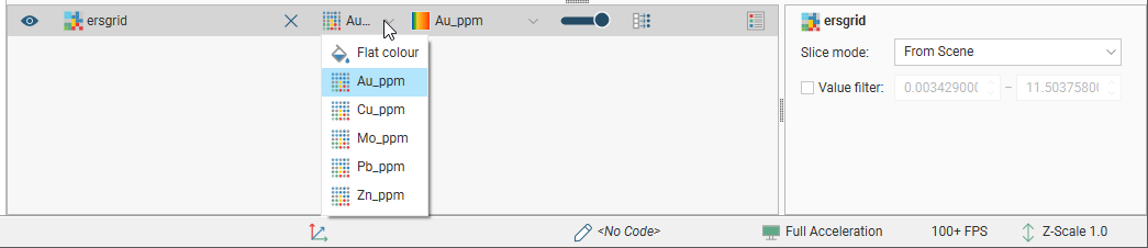
Grids can be displayed as points (![]() ) or as cells and the values filtered, as described in Displaying Points.
) or as cells and the values filtered, as described in Displaying Points.
3D Grids
Leapfrog Works imports the following types of 3D grids:
- GOCAD Voxet Files (*.vo)
- Geosoft Voxels (*.geosoft_voxel)
- Magnetotelluric Resistivity (OUT) Files (*.out, *.out.gz, *.mod) (with the Geophysics extension)
- UBC Mesh Files (*.msh)
To import these 3D grid types, right-click on the Geophysical Data folder and select Import 3D Grid. Leapfrog Works will ask you to specify the file location. Click Open to start importing the grid. Further information about importing each grid type is discussed below. See:
- Importing GOCAD Models
- Importing Geosoft Voxels
- Importing Magnetotelluric Resistivity Files (with Geophysics extension)
- Importing UBC Grids
Once in Leapfrog Works, you can evaluate geological models, interpolants and distance functions in the project on the grid. You can also import UBC properties for each of these grid types, and 3D grids can be exported in CSV, UBC or Geosoft voxel formats. See:
- Importing UBC Properties
- Exporting 3D Grids in CSV Format
- Exporting 3D Grids in UBC Format
- Exporting 3D Grids in Geosoft Voxel Format
Importing GOCAD Models
Leapfrog Works imports GOCAD Voxet files in *.vo format. To do this, right-click on the Geophysical Data folder and select Import 3D Grid. In the window that appears, select the file you wish to import and click Open.
In the window that appears, the number of blocks in the file is displayed. If you wish to select only a subset of the blocks, increase the Subsample Rate.
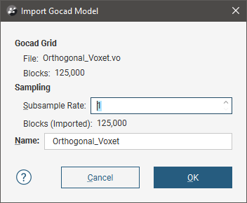
Click OK to import the grid, which will appear in the Geophysical Data folder.
Importing Geosoft Voxels
Leapfrog Works imports Geosoft Voxel files in *.geosoft_voxel format. To do this, right-click on the Geophysical Data folder and select Import 3D Grid. In the window that appears, select the file you wish to import and click Open.
In the window that appears, enter a different name for the grid, if required, then click OK. The grid will be added to the Geophysical Data folder.
Importing Magnetotelluric Resistivity Files
Importing magnetotelluric resistivity (OUT) files requires the Geophysics extension.
Leapfrog Works imports magnetotelluric resistivity (OUT) files in *.out, *.out.gz and *.mod formats. To do this, right-click on the Geophysical Data folder and select Import 3D Grid. In the window that appears, select the file you wish to import and click Open.
In the window that appears, choose whether or not you will apply a threshold.
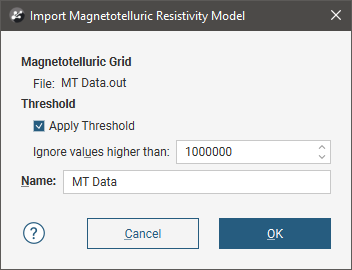
Click OK to import the grid, which will appear in the Geophysical Data folder.
Importing UBC Grids
Leapfrog Works imports UBC grids in *.msh format, together with numeric values in properties files in *.gra, *.sus, *.mag and *.den formats. To do this, right-click on the Geophysical Data folder and select Import 3D Grid. In the window that appears, select the file you wish to import and click Open.
Next, a window will appear in which you can add any property files you also wish to import, although these are not required. Click on the (![]() ) button and select the files you wish to import:
) button and select the files you wish to import:
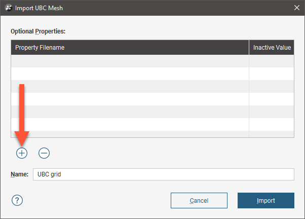
You can add more properties files to the grid once it has been imported.
Click Import. The grid will be added to the Geophysical Data folder.
Importing UBC Properties
To import UBC properties for an existing 3D grid, right-click on the grid in the project tree and select Import UBC properties. In the window that appears, select the file you wish to import and click Open. You will be prompted to set the Inactive Value field to mark cells as inactive. Doing so does not change the data but ensures that cells with the inactive value can be hidden when the grid is displayed in the scene.
Click OK. The data column will be added to the grid.
Exporting 3D Grids in CSV Format
3D grids can be exported in CSV format. To do this, right-click on the grid in the project tree and select Export. Leapfrog Works will step you through a series of options for exporting the grid.
Choose which evaluations, calculations and filters will be included in the exported file. Items added to the Selected items list will appear in the exported file as columns, and the order of columns in the file will match the order shown in the project tree.
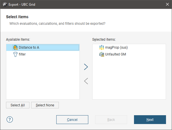
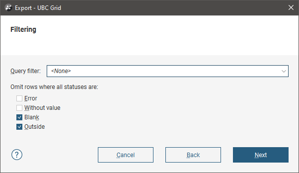
There are two options for filtering out rows:
- Use a Query filter to filter rows out of the data exported. Note that this is different from exporting filters as columns in the Select Items step.
- The Omit rows... options are useful when all block results are consistently the same non-Normal status. Select from Error, Without value, Blank or Outside; all rows that consistently show the selected statuses will not be included in the exported file.
To change either the Centroid and size precision and Value precision options, untick the box for Use default precision and select the required option.
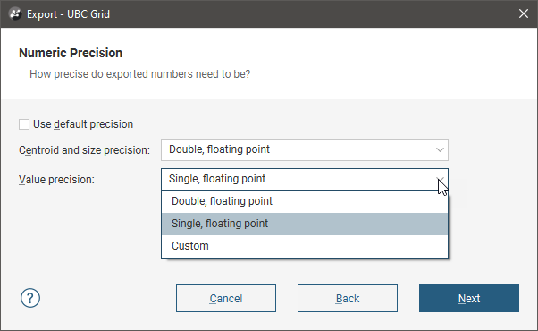
There are three encoding options:
- The Double, floating point option provides precision of 15 to 17 significant decimal places.
- The Single, floating point option provides precision of 6 to 9 significant decimal places.
- The Custom option lets you set a specific number of decimal places.
When a 3D grid is exported, non-Normal status codes can be represented in the exported file using custom text sequences.
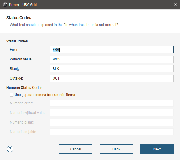
The Status Codes sequences are used for category status codes and filter status codes exported as columns. For filter status codes, Boolean value results will show FALSE and TRUE for Normal values or the defined Status Codes for non-Normal values.
Numeric Status Codes can be represented using custom text sequences. This is optional; if no separate codes are defined for numeric items, the defined Status Codes will be used.
The selection you make will depend on the target for your exported file. You can choose a character set and see what changes will be made:
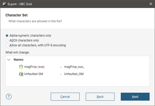
Once you have made any Character Set changes, click Next to view a summary of the selected options.
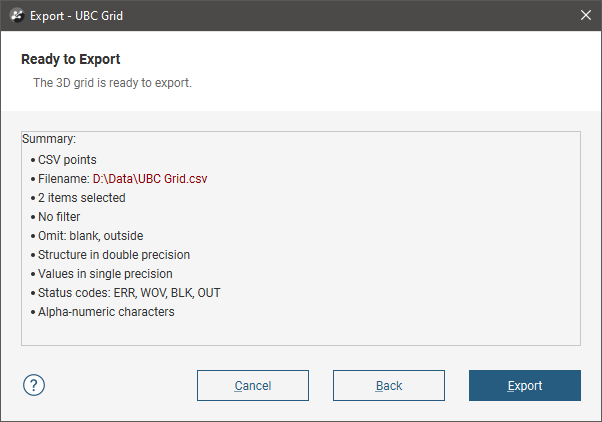
If you need to make any changes, you can work back through the steps.
Once you’re satisfied with the settings chosen, click Export to save the file.
The selections you make when you export a 3D grid will be saved. This streamlines the process of subsequent exports of the grid.
Exporting 3D Grids in UBC Format
3D grids can be exported in UBC format. To do this, right-click on the grid in the project tree and select Export as UBC Grid.
When a 3D grid is exported in UBC format with a category evaluation, category data is mapped to an editable numeric value. If the grid has any category evaluations, you will first be prompted to check the numeric values used for each category:
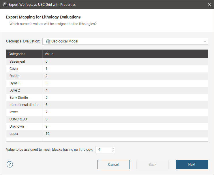
Double-click on a value to edit it. You can also change the value assigned to blocks that have no lithology.
Click Next to select the properties you wish to export and edit the file names used, if required.
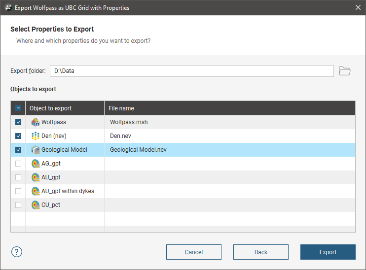
If the grid has no category evaluations, this is the first window that will appear when you select the Export as UBC Grid option.
Click Export to save the files.
Exporting 3D Grids in Geosoft Voxel Format
3D grids can be exported in Geosoft Voxel format. To do this, right-click on the grid in the project tree and select Export as Geosoft Voxels. In the window that appears, select the properties you wish to export and edit the file names used, if required.
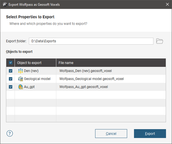
Click Export to save the files.
2D and 2D Crooked SEG-Y Data
Importing 2D SEG-Y data requires the Geophysics extension.
Leapfrog Works imports 2D and 2D crooked SEG-Y data in *.segy and *.sgy formats. External navigation files are not supported.
To import 2D SEG-Y data, right-click on the Geophysical Data folder and select Import 2D SEG-Y. Leapfrog Works will ask you to specify the file location. Click Open to start importing the file.
Leapfrog Works will read the data in the file and match the data to the expected format. In most cases, Leapfrog Works will set the correct values from the information in the file.
There are two steps to work through. First, set up the Key Field Locations. There are buttons at the top of the window for displaying the Text Header and Binary Header, which may be useful in deciding what import settings to use.
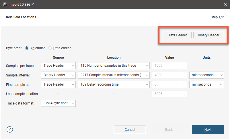
You can keep the Text Header and Binary Header windows open while you work through the steps in the Import 2D SEG-Y window.
Settings for the Key Field Locations are:
- Byte order. This will be Big endian or Little endian and must be correct in order for the other data in the file to be read correctly.
- Samples per trace. This is the number of samples in each trace. If the correct value cannot be read from the file, you can set it manually by selecting User from the Source dropdown list.
- Sample interval. This is the vertical sample spacing for the trace data and is almost always stored in thousandths of true units. If the correct value cannot be read from the file, you can set it manually by selecting User from the Source dropdown list.
- First sample at. This is the delay recording time for the first sample. If the correct value cannot be read from the file, you can set it manually by selecting User from the Source dropdown list.
- Last sample location. This is read-only and is the calculated location from the last sample in the trace.
- Trace data format. This should be defined in the binary header.
Click Next to move on to setting the Coordinate Field Locations. In this step, the More button displays the trace header fields:
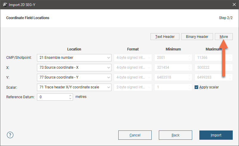
Settings for the Coordinate Field Locations are:
- Inline. This is the location in the trace header of the in-line coordinate.
- Crossline. This is the location of the cross-line location.
- X. This is the location of the X-coordinate of the trace location.
- Y. This is the location of the Y-coordinate of the trace location.
- Scalar. This the coordinate scale factor used for ground coordinates. It is read-only, but you can choose to disable the scalar by disabling the Apply scalar option.
Use the Reference Datum field to specify the file’s elevation.
When you are finished, click Import. The file will appear in the Geophysical Data folder.
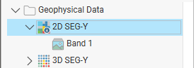
In the project tree, the file is organised into the main data object and the colour band object. Drag either one into the scene to view the data.
3D SEG-Y Data
Importing 3D SEG-Y data requires the Geophysics extension.
Leapfrog Works imports 3D SEG-Y data in *.segy and *.sgy formats.
To import 3D SEG-Y data, right-click on the Geophysical Data folder and select Import 3D SEG-Y. Leapfrog Works will ask you to specify the file location. Click Open to start importing the file.
Leapfrog Works will read the data in the file and match the data to the expected format. In most cases, Leapfrog Works will set the correct values from the information in the file.
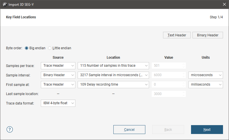
There are four steps to work through. In the last step, you can choose how many slices to import. First, set up the Key Field Locations. There are buttons at the top of the window for displaying the Text Header and Binary Header, which may be useful in deciding what import settings to use.
You can keep the Text Header and Binary Header windows open while you work through the steps in the Import 3D SEG-Y window.
Settings for the Key Field Locations are:
- Byte order. This will be Big endian or Little endian and must be correct in order for the other data in the file to be read correctly.
- Samples per trace. This is the number of samples in each trace. If the correct value cannot be read from the file, you can set it manually by selecting User from the Source dropdown list.
- Sample interval. This is the vertical sample spacing for the trace data and is almost always stored in thousandths of true units. If the correct value cannot be read from the file, you can set it manually by selecting User from the Source dropdown list.
- First sample at. This is the delay recording time for the first sample. If the correct value cannot be read from the file, you can set it manually by selecting User from the Source dropdown list.
- Last sample location. This is read-only and is the calculated location from the last sample in the trace.
- Trace data format. This should be defined in the binary header.
Click Next to move on to setting the Coordinate Field Locations. In this step, the More button displays the trace header fields:
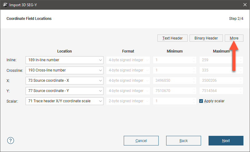
Settings for the Coordinate Field Locations are:
- Inline. This is the location in the trace header of the in-line coordinate.
- Crossline. This is the location of the cross-line location.
- X. This is the location of the X-coordinate of the trace location.
- Y. This is the location of the Y-coordinate of the trace location.
- Scalar. This the coordinate scale factor used for ground coordinates. It is read-only, but you can choose to disable the scalar by disabling the Apply scalar option.
Click Next to move on to setting the Tie Points. By default, these are calculated from the trace headers, but if they are not in the trace headers or if you have more precise values from the text header or from another source, click User supplied and entering these values manually.
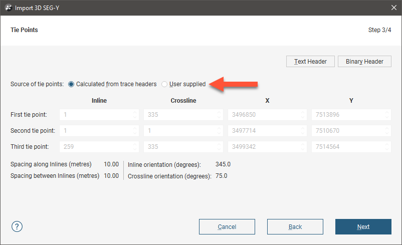
The Spacing along Inlines and Spacing between Inlines fields are calculated from the specified tie points.
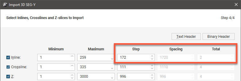
Click Next to move on to selecting the slices you will import. The Total column tells you the number of in-lines, cross-lines and z-slices that will be imported.
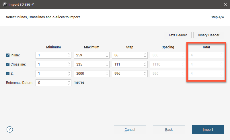
If you wish to import fewer or more slices, adjust the Minimum, Maximum or Step values, and the Total number of slices will be updated:
Once you have imported 3D SEG-Y data into a Leapfrog Works project, you can add more slices and delete existing slices if you need to. This is described below.
Use the Reference Datum field to specify the file’s elevation.
When you are finished, click Import. The file will appear in the Geophysical Data folder.
In the project tree, the file is organised into an extents object and separate folders for the in-lines, cross-lines and z-slices:
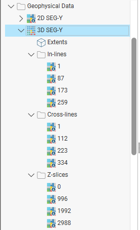
You can drag slices into the scene one-by-one or display, say, all z-slices by dragging the Z-slices folder into the scene.
To delete slices, right-click on them and click Delete.
If you wish to add more slices, right-click on the data object and select Import More Slices:
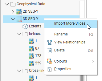
This launches the Import 3D SEG-Y window once again and you can select additional slices by changing the Minimum, Maximum or Step values in the last step.
Got a question? Visit the Seequent forums or Seequent support
© 2023 Seequent, The Bentley Subsurface Company
Privacy | Terms of Use