
Importing Drilling Data
Leapfrog Energy can import drilling data from the following sources:
- Files stored on your computer or a network location
- From a Central project’s Data Room
- From any database that runs an ODBC interface
- From an acQuire database
For each of these options, once the data source is selected, the process of importing drilling data is the same. See Importing Data Tables and Mapping Data Columns in the Working With Data Tables topic for an overview of how to map data columns in files to the format Leapfrog Energy expects.
The rest of this topic discusses the data format required for importing drilling data, how to connect to different data sources, how to add more tables to a drilling data set and the well desurveying options available in Leapfrog Energy. It is divided into:
- Expected Drilling Data Tables and Columns
- AGS Format Drilling Data
- Importing Drilling Data From the Central Data Room
- Connecting to an ODBC Data Source
- Connecting to an acQuire Database
- Importing Well Deviation Files
- Setting Elevation for Collar Points
- Desurveying Options
Expected Drilling Data Tables and Columns
Required table types for importing drilling data are:
- A collar table
- A survey table
- At least one interval table
Downhole points tables can also be imported, but are optional.
A screens table can also be imported but is optional.
The following formats are supported:
- AGS Files (*.ags)
- ASCII Text Files (*.asc)
- CSV Text Files (*.csv)
- Data Files (*.dat)
- Plain Text Files (*.txt)
- TSV Text Files (*.tsv)
For data imported in CSV, ASCII, TXT, DAT and TSV formats, separate files are required for each type of table. For data imported in AGS format, a single file is imported that contains each type of table and a summary of the relevant data is presented at each stage of the importation process so you can select from the available groups of data. AGS format is described in AGS Format Drilling Data below.
The Collar Table
The collar table should contain five columns:
- A well identifier
- The location of the well in X, Y and Z coordinates
- The maximum depth of the well
A collar table can also contain a trench column, and collars marked as trenches will be desurveyed in a manner different from other wells. See Desurveying Options for more information.
Leapfrog Energy expects a 0 for a normal hole and a 1 for a trench. If there is no trench column in the collar table, Leapfrog Energy will create one.
The well ID is used to associate data in different tables with a single well. The ID for a well must be identical in all tables in order for data to be associated with that well. Inconsistencies in the way wells are identified are common sources of errors.
The maximum depth column is optional. If it is present, is used to validate the data imported for the interval tables. The maximum depth specified is often a planned quantity, whereas the interval table records actual measurements. For this reason, Leapfrog Energy has an option for fixing the maximum depth value in the collar table to match the data in an interval table.
If maximum depth information is not included in a collar file, Leapfrog Energy will determine it from the maximum depth sampled as indicated by data in the interval tables.
The Survey Table
For the survey table, Leapfrog Energy expects a minimum of four columns:
- A well identifier
- Depth, dip and azimuth values
For the survey table, Leapfrog Energy expects a well identifier and depth, dip/inclination and azimuth values. You cannot have both an inclination column and a dip column so if a table contains both columns, you will need to choose between the two. When you import an inclination column, the survey table in the project tree will include a dip column, calculated from the inclination values.
By default, Leapfrog Energy assumes that negative dip values point up. If this is not the case, tick the Negative survey dip points down option.
See Desurveying Options for more information on the well desurveying algorithms used in Leapfrog Energy.
The Screens Table
For the screens table, Leapfrog Energy expects a minimum of four columns:
- A well identifier
- Start/from and end/to depths
- A value column
Interval Tables
For interval tables, Leapfrog Energy expects, at minimum, four columns:
- A well identifier
- Start/from and end/to depths
- A column of measurements
If a well ID in an interval table does not correspond to one in the collar table, the table can still be imported but the interval table will contain errors.
Supported column types are:
- Lithology columns containing lithologic data, which can be used for geological modelling.
- Numeric columns containing numeric values, which can be used for interpolating data.
- Category columns, which is text representing categories such as company, geologist, or mineralisation.
- Text columns containing text data that is not categorical, such as comments. Text columns are not validated when imported.
- Date columns containing date data. Custom date and timestamps formats are supported.
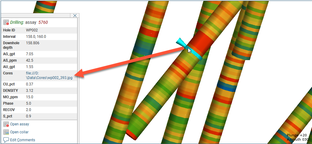
- URL columns. Use the prefix file:/// to link to local files.
- Hex colour columns containing RGB triplets.
When an interval table is displayed in the scene and an interval is selected, clicking on a link in the URL column will open the link. This is a useful way of linking to, for example, data files or core photo images from within Leapfrog Energy:
Points Tables
For downhole points tables, Leapfrog Energy expects the following columns:
- A well identifier
- Depth
AGS Format Drilling Data
Leapfrog Energy supports the importation of drilling data using the Association of Geotechnical and Geoenvironmental Specialists (AGS) format. AGS versions 3.1 and 4 are supported. The process for importing boreholes in AGS format is the same as that for importing data described in the rest of this topic, except that a single file is selected for import.
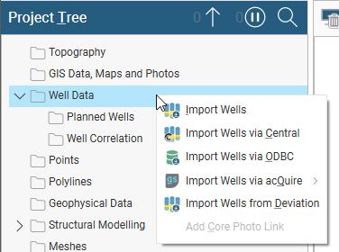
To import drilling data in AGS format, right-click on the Well Data folder and select where you wish to import the data from. In the Import Wells window, click the button for Collar to locate the file you wish to use.
For each type of table, a summary of the relevant data in the file is presented, allowing you to select groups of data.
The Collar Table
For the collar data group, the HOLE group (v 3.1)/LOCA group (v 4.0) will automatically be selected. Click OK to accept the selection, then check how the selected data has been mapped.
The Survey Table
For the survey table data group, the HOLE group (v 3.1)/HORN group (v 4.0) will automatically be selected. Click OK to accept the selection.
Interval Tables
All remaining groups that contain suitable interval data are displayed, although you can display all groups in the file by disabling the Only show groups suitable for interval data option.
Only one group can be selected, and typically the GEOL table contains the lithology data. However, if you need to import more groups, there are two options:
- Import the other groups as additional interval tables (see Importing Drilling Data). Select Import From File and then select whether you wish to import intervals or points, then select the AGS file again.
- Append the data set, as described in Adding New Rows to Existing Data Tables in the Working With Data Tables topic.
Depth Points Tables
All remaining groups that contain points data are displayed, although you can display all groups in the file by disabling the Only show groups suitable for depth points data option.
Importing Drilling Data From the Central Data Room
Drilling data can only be imported from a project’s data room. Although drilling data can be published to Central, that is for the purpose of visualising the data in the Central Portal. Published drilling data cannot be imported into other Leapfrog Energy projects.
See the Storing and Accessing Data in the Project Data Room topic in the Central help for information on how to work with a Central project’s data room.
To import drilling data from Central, first make sure you are connected to a Central server. Next, click on the Well Data folder and select Import Wells via Central. In the window that appears, select the project you wish to import data from. The Import Wells from Central window will be displayed. Click the button for Collar to navigate the project’s data room to locate the collar file you wish to use.
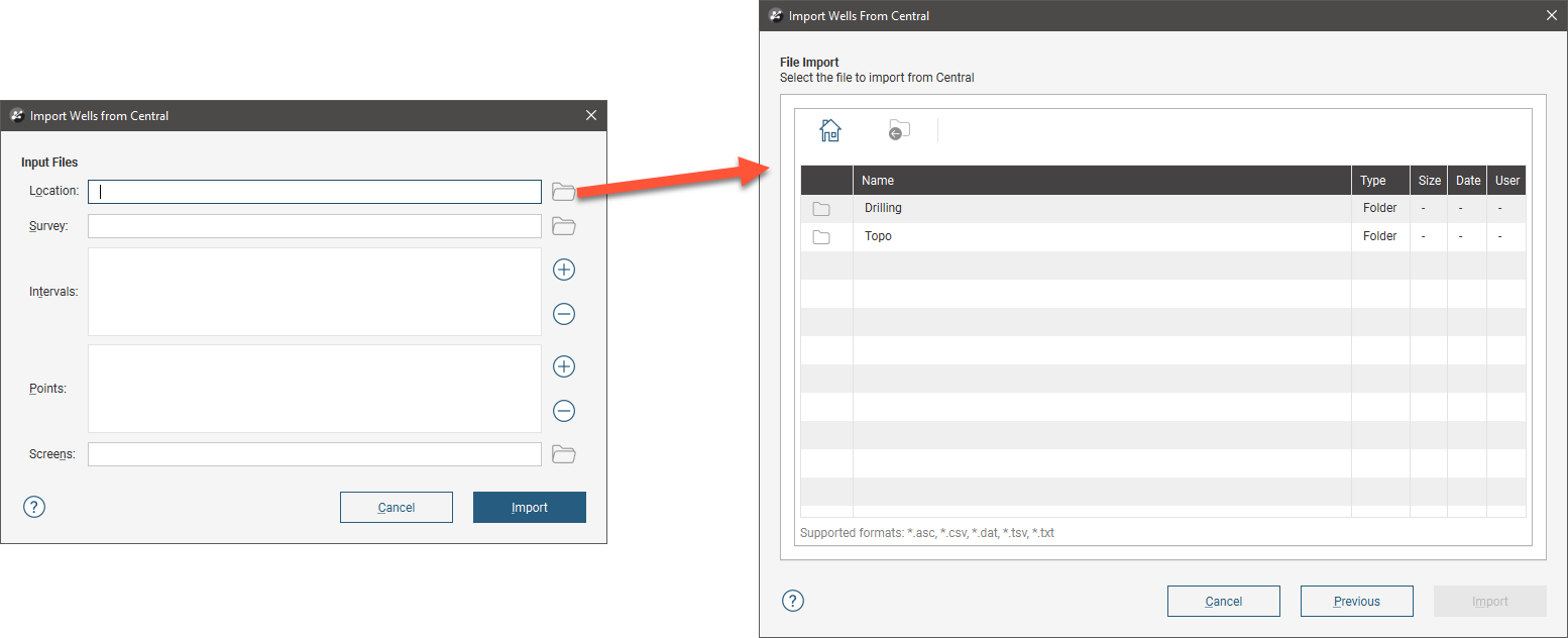
Select the file and click Import. Work through the files as described in Importing Data Tables and Mapping Data Columns.
Connecting to an ODBC Data Source
Leapfrog Energy supports database files in Access Database (*.mdb, *.accdb) formats.
To import drilling data directly from any database that uses an ODBC interface, right-click on the Well Data folder and select Import Well Data via ODBC. The Select ODBC Data Source window will appear:
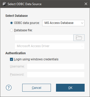
Enter the information supplied by your database administrator and click OK.
If you are importing from a local database file, click the Database file option and then browse to locate the file.
Selecting Tables
In the Select Tables To Import window, select the tables you wish to import.
To add an interval or points table, click the Add button (![]() ); the list of tables in the database will be displayed. To remove a table from either list, click on it and click the Remove button (
); the list of tables in the database will be displayed. To remove a table from either list, click on it and click the Remove button (![]() ).
).
Click OK to begin the process of importing the data. Work through the files as described in Importing Data Tables and Mapping Data Columns.
Connecting to an acQuire Database
There are two options for connecting to an acQuire database:
- Create a new connection. To do this, right-click on the Well Data folder and select Import Well Data via acQuire > New Selection. Select the server and click Connect. Next, enter the login details supplied by your database administrator.
- Create a connection from an existing selection file. Right-click on the Well Data folder and select Import Well Data via acQuire > Existing Selection. Navigate to the location where the selection file is stored and open the file.
Once connected to the database, you will be able to select the required data using the Select data from acQuire window.
Optionally, click the Profiles button and choose a profile from those on the acQuire database. Profiles are created in acQuire; see your acQuire administrator for more information.
You can also use the other tabs on the acQuire component interface to make other data selections.
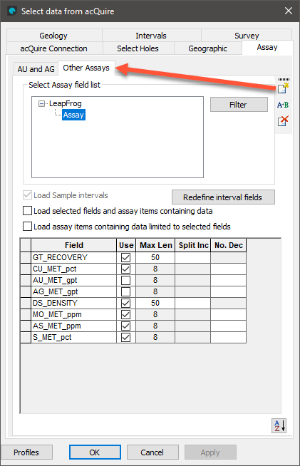
In the Select data from acQuire dialog provided by the acQuire component, both the Geology and Assay tabs can have additional pages added to select different sets of fields. To add a page, click the Create new page button. Each page will end up as a separate interval table under the Wells object in the project tree.
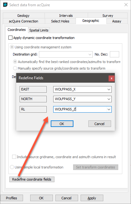
To successfully import data from some acQuire databases, it may be necessary to redefine the coordinate fields using the Refine coordinate table button on the Geographic tab.
For more information on using the third-party selection tools provided in the Select data from acQuire window, see your acQuire user documentation. When you have finished specifying the selection, click OK to import the data.
Once the drilling data has been loaded, you can:
- Import additional interval tables. See Importing Drilling Data below.
- Update the drilling data with new data from the acQuire database. See Smart Refresh below.
- Reload drilling data. See Reloading Data Tables in the Working With Data Tables topic.
Add Additional Columns
To add a column for a collar or a survey table, right-click on the table in the project tree and click Import Column. To add a column for an interval table, right-click on the interval table in the project tree and click New Column > Import Column.
Having set up an acQuire database to provide drilling data, you can add columns that were not previously imported to tables without deleting a table and reimporting it. This is useful if a particular column was not available in acQuire at the time the database connection was established, or it was previously thought a particular column was not needed and was left unticked when the database import was configured.
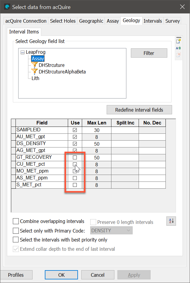
In the acQuire import component’s window, select either the Assay or Geology tabs and tick Use next to any Field you want to appear as an available column that has not previously been selected for import, then click Apply and OK.
When the Add Table Column From acQuire window opens, select columns to import into Leapfrog Energy. Such columns may be ones that have only just been made available via the step above, or may have been ones already available for import from the acQuire database that were not previously selected for import in the Add Table Column From acQuire window.
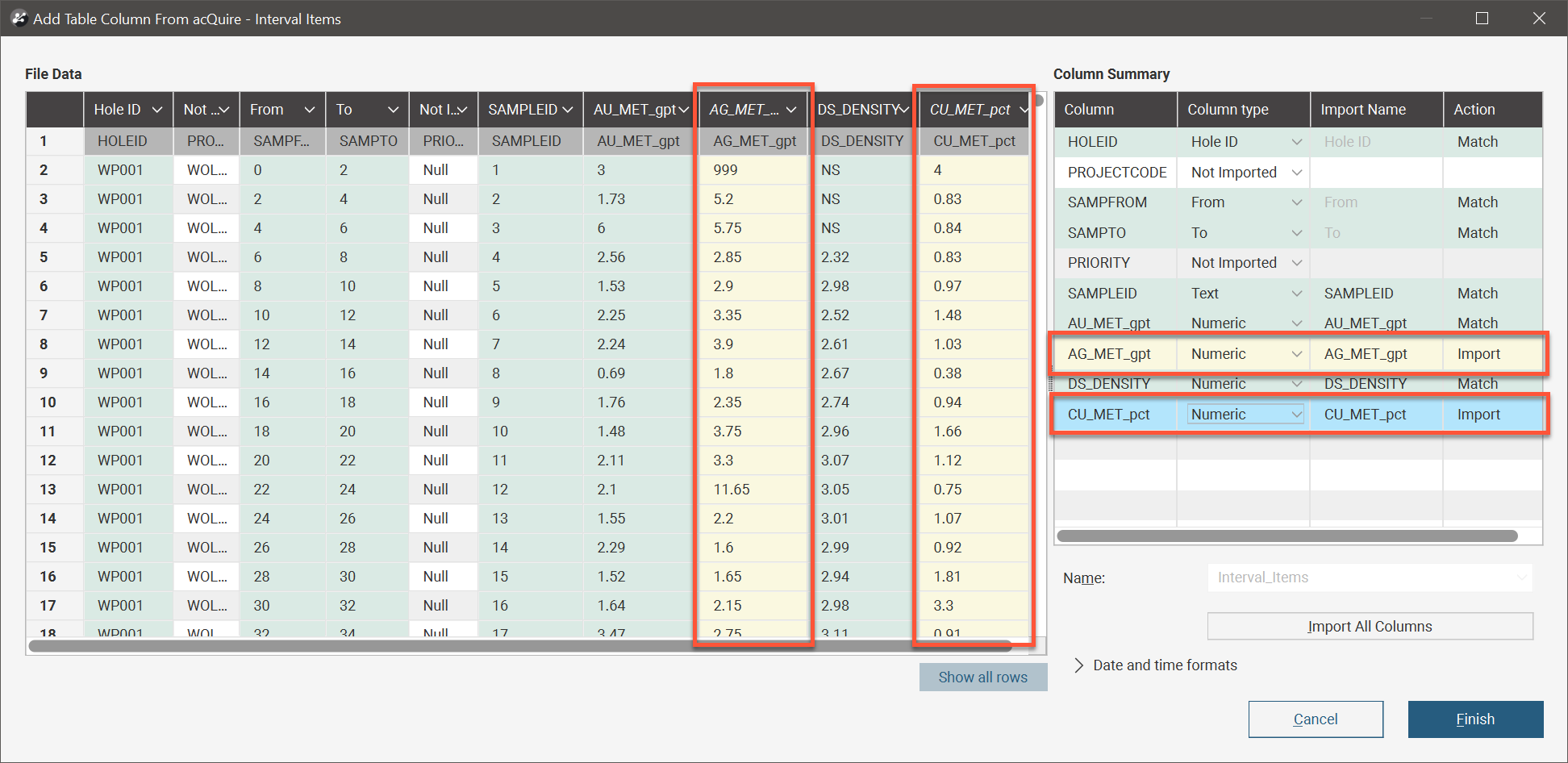
Select the Column type for the data columns being imported and click Finish. The newly added columns will appear in the project tree under the selected table.
Smart Refresh
Smart Refresh obtains the latest drilling data from the acQuire database without reloading the entire contents of the database. This reduces the amount of data transfer required and speeds data updated. If any data relating to a well has changed, the whole well is updated. Any new wells in the database can be added.
Right-click on the drilling data set in the project tree and select Smart Refresh. If no structural differences are noted between the source and the imported table, you will be given the choice to import all tables automatically, and the previous import settings will be reused in executing the refresh. Alternatively, you can choose the Import Manually option, which will step through the import tables dialog windows. If structural differences will cause a problem with the refreshed import, you will be warned that there is a Problem refreshing the table and you can Cancel or Import Manually. You can also click Show full error message to get more information on the problem detected.
Saving a Selection
Saving a selection saves the current acQuire database selection to file for future reuse. You can use a selection to import the same set of drilling data in new Leapfrog Energy projects.
To save an acQuire selection, right-click on the drilling data set in the project tree and select Save Selection. You will be prompted for a filename and location.
Importing Well Deviation Files
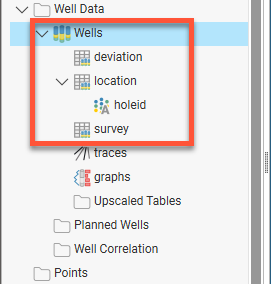
Leapfrog Energy supports the importation of drilling data in Petrel deviation file format. Each well in the drilling data set is stored in a separate *.dev file that has a header containing the well ID and the x-y-z location of the top of the well. Leapfrog Energy uses the information in each file to build a drilling data set organised into a deviation table, a location table and a survey table:
The following columns are required in each *.dev file:
- Measured depth (MD)
- Downhole X, Y and Z columns for the desurveyed coordinates
- True vertical depth (TVD)
Leapfrog Energy calculates the survey data from the downhole locations and so dip and azimuth columns are not required.
To import deviation files, right-click on the Well Data folder and select Import Wells from Deviation. In the window that appears, select the files you wish to import, then click Open. Work through the file importer as described in the Importing Data Tables and Mapping Data Columns topic.
Because each table in the drilling data set it made up of data in separate *.dev file, you cannot remap the data source for well deviation files.
If the source data changes, there are two options:
- Appending the data
- Reloading the data
Which option you choose depends on how the source data has changed.
Appending Well Deviation Files
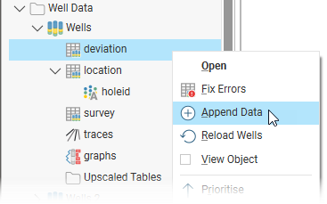
Appending the data adds new data to Leapfrog Energy without overwriting the existing data. If there are new wells available, i.e. additional *.dev files, and you do not wish to change the data already in the project, use the Append Data option to add the new wells to the drilling data set. To do this, right-click on the deviation table and select Append Data:
In the window that appears, select the files you wish to add to the data set, then click Open. Leapfrog Energy will process the files and add them to the existing data set without changing any information already in the project. Note that if you have accidentally selected files for wells that are already in the project, data for those wells will remain unchanged in the project.
Reloading Well Deviation Files
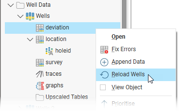
If the data already in Leapfrog Energy has been changed outside the project and, perhaps, there are new wells, use the Reload Wells option to overwrite the data already in Leapfrog Energy and add wells defined in any new *.dev files. To do this, right-click on the deviation table and select Reload Wells:
In the window that appears, select the files you wish to include in the data set.
Note that only the wells you select will appear in the reloaded data set, so be sure to also select the files for the wells already in the project, if you wish to retain them.
Click Open. Leapfrog Energy will process the files selected and update the drilling data set.
Setting Elevation for Collar Points
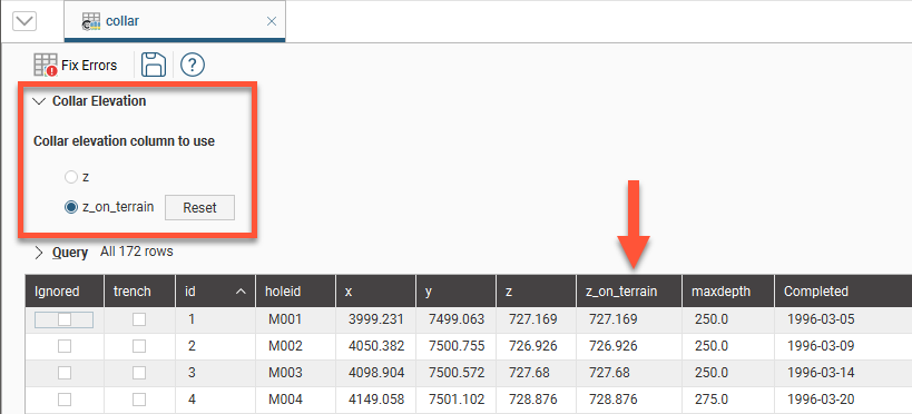
You can set the elevation for all collar points or for a subset of collar points by projecting them onto a surface. This creates a new column in the collar table called z_on_terrain, and you can switch between using the original values in the z column and the projected values in the z_on_terrain column:
To set the elevation for collar points from a surface, right-click on the collar table in the project tree and select Set Elevation. The Set Elevation from Surface window will appear:
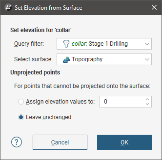
Select from the surfaces available in the project and set a query filter, if you wish to limit the collars you will project onto the surface.
If the surface does not intersect vertically with some points, you can choose how the z_on_terrain values for those points will be determined. There are two options:
- Assign elevation values to sets the z values to a fixed elevation for all unprojected points.
- Leave unchanged makes no changes to the z values for unprojected points; the original z column values will be used.
Click OK to set elevation values.
The collar table will be updated with an additional column, z_on_terrain:
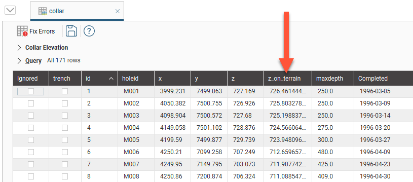
The z_on_terrain column values are determined as follows:
- For selected points that can be projected onto the surface, the elevation values from that surface are used
- For points that cannot be projected onto the surface, either a fixed elevation value or the original values from the z column are used, depending on the chosen Unprojected points option.
- For points you have chosen not to project, i.e. if you have used a query filter, the original values from the z column are used.
The original z values are preserved in the z column. To switch back to the original z values, click on Collar Elevation, then select the original column:
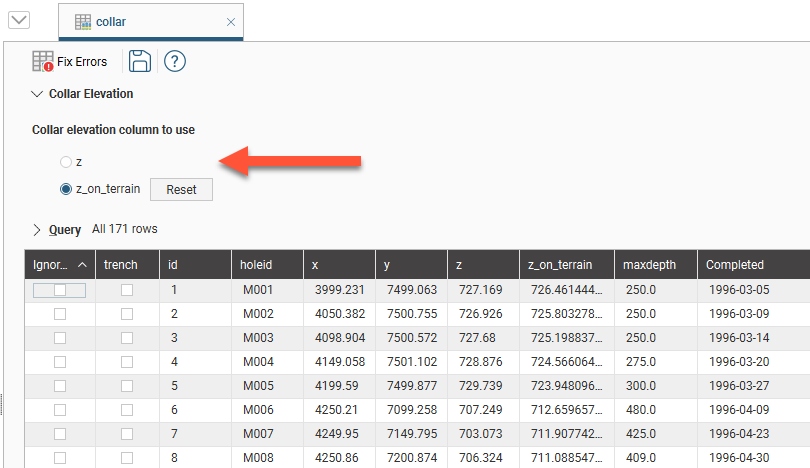
The z_on_terrain column will remain in the collar table; switching to using the original z column does not delete the z_on_terrain column.
Applying a query filter is useful for limiting the collars projected onto a surface. Here, a query filter has been used to project a single collar, M005, onto the topography:
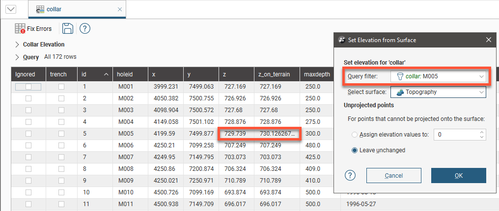
All other values in the z_on_terrain are from the z column.
Note that you can repeat this process for multiple subsets of collar points, if there are different surfaces you wish to use in setting the elevation for different subsets of points.
If the collar table is reloaded:
- For existing wells, z_on_terrain values are not overwritten on reload.
- For new wells added during the reload, the z_on_terrain value will be left blank.
- For an existing well that has a changed z value, the z_on_terrain will remain unchanged on reload.
You can also clear the projected values from the z_on_terrain column by clicking the Reset button, in which case the z_on_terrain column will be reset to the z column values:
Desurveying Options
Well desurveying computes the geometry of a well in three-dimensional space based on the data contained in the survey table. Under ideal conditions, the well path follows the original dip and azimuth established at the top of the well. Usually, though, the path deflects away from the original direction as a result of layering in the rock, variation in the hardness of the layers and the angle of the drill bit relative to those layers. The drill bit will be able to penetrate softer layers more easily than harder layers, resulting in a preferential direction of drill bit deviation.
There are a number of paths a well could take through available survey measurements, but the physical constraints imposed by drilling are more likely to produce smoother paths. Selecting the desurveying method that gives the best likely approximation of the actual path of the well will ensure that subsequent modelling is as accurate as possible.
Leapfrog Energy implements three algorithms for desurveying wells:
These options are described in more detail below.
If downhole survey data is missing, Leapfrog Energy will continue the well trace in a straight line in the last known direction. This is because Leapfrog Energy assumes that the reason no further survey data was recorded was that there were no subsequent direction changes.
Another factor that affects how wells are desurveyed is how dip values are handled. When the survey table is imported, Leapfrog Energy sets the Negative survey dip points down value according to the data in the imported table. When the majority of the dip data in the table is positive, Leapfrog Energy assumes all these wells will point down and leaves the field Negative survey dip points down disabled. When most of the values are negative, the field is enabled. This field can be changed by double-clicking on the survey table to open it and then clicking on Compatibility to show the table’s desurveying settings:
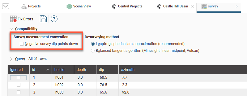
If you are going to change the automatically set value of Negative survey dip points down, consider carefully the implications if there is a mix of wells pointing down and up.
The other Compatibility setting relates to the algorithm used in desurveying the wells.
The Spherical Arc Approximation Algorithm
The default algorithm used in Leapfrog Energy is spherical arc approximation, which is sometimes referred to as the minimum curvature algorithm. Downhole distances are desurveyed exactly as distances along a circular arc:
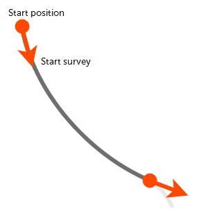
The algorithm matches the survey at the starting and end positions exactly and the curvature is constant between these two measurements. At the survey points, the direction remains continuous and, therefore, there are no unrealistic sharp changes in direction.
If you wish to use spherical arc approximation, there is no need to change any settings.
The Balanced Tangent Algorithm
The balanced tangent algorithm uses straight lines but attempts to improve the accuracy of the raw tangent algorithm by assigning equal weights to the starting and end survey measurements:
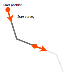
It is an improvement on the raw tangent algorithm but still suffers from an unrealistic discontinuity in the well path. It is, however, a better approximation of the overall well path and is reasonably accurate when the spacing between measurements is small.
To use the balanced tangent algorithm, double-click on the survey table in the project tree. Click on Compatibility and change the Desurveying method.
The Raw Tangent Algorithm
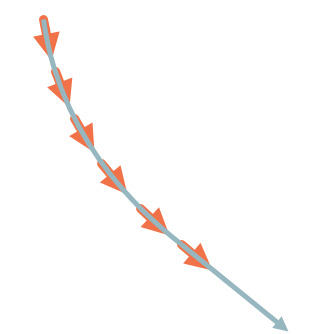
The raw tangent algorithm assumes the well maintains the direction given by the last survey measurement until the next new measurement is reached:
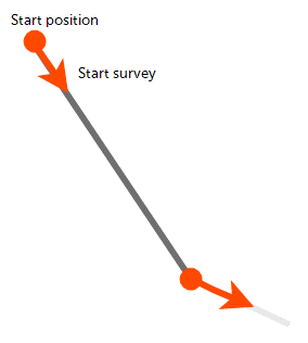
This implies that the well makes sharp jumps in direction whenever a measurement is taken, which is unlikely, except when the well is being used to define a trench.
Collar tables have a trench column that indicates whether or not the well is from a trench. When the trench column is ticked for a well, the trench will be desurveyed using the raw tangent algorithm. Double-click on the collar table in the project tree, then tick the trench box for the wells you wish to desurvey using the raw tangent algorithm.
Got a question? Visit the Seequent forums or Seequent support
© 2023 Seequent, The Bentley Subsurface Company
Privacy | Terms of Use