Display Grid

Use the Overlay > Grids and Images > Display a Grid menu option to display a georeferenced level plan or vertical section grid in a GM-SYS Profile model pane.

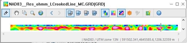
2D SEG-Y profiles are created (using the SEG-Y Importer) as crooked section Vertically gridded profile data is frequently collected, extracted, or calculated along a line that has a non-straight path; such data is displayed in Oasis montaj using a specially defined grid orientation called a crooked section. grids. You can visualize your seismic data by importing these section grids into your GM-SYS Profile model. A crooked section grid is projected perpendicularly onto a flat section map within your model and is displayed in either the Depth or the Time pane. For more details on crooked section grids, see the Application Notes below.

Display Grid dialog options

Grid name	Select the grid file to display.
Orientation	Contextual, read-only parameter that will display: "none" – if the selected grid does not have an orientation or no grid is yet selected. "Crooked Section" – if the selected grid is a crooked section grid. "Section, Azimuth: Origin: " – if the selected grid is a section oriented grid. "Level Plan, Depth: " – if the selected grid is a plan oriented grid.
Colours	Select the colour scheme for rendering the image of the selected grid. If you mouse over the colour ramp entry, a tool tip will display the name of the colour table file. To modify the selection, click on the colour entry and then navigate through the scheme categories.
Colour method	Select the colour method. If the selected colour scheme is an .itr file or a .zon file, the colours are already attributed to data ranges, and this entry remains disabled. The colour method can be one of: As last displayed Default Histogram equalization Normal distribution Linear Log-linear The method "As last displayed", will display each grid as it was displayed the last time the grid was viewed, and the colour tables will be ignored.
Target pane	Select the pane on which to draw the selected grid: Plan View (section oriented grids, images, and crooked section grids are not supported) Depth Section (plan oriented grids and images are not supported) Time Section (plan oriented grids and images are not supported) If the selected pane is incompatible with the orientation of the grid, a validation error will be shown.
Brightness	The normal brightness is defined at 0. You can change the brightness from -100 (black) to 100 (white) using either the slider bar or by entering an exact value.
Reverse colour distribution	The colour table can be used in reverse order. Check this box to reverse the order. For example, the colour table for displaying resistivity data is the inverse of the one used for conductivity. By allowing to reverse the colour table on the fly, the same table can be used to display both.
Smoothing	For display purposes, by default, the grid is first interpolated to a smooth image at the screen resolution. If you prefer to honour the grid resolution, leave the Smoothing option unchecked: the image will appear pixelated, and the colour will change at the actual grid interval rather than the screen resolution.
Shading	Adding a shading effect to the colour grid emphasizes the subtle changes in the data that would otherwise be subdued. Presenting the data shaded is optional. Check this option to shade the colour grid image. If checked, by default the sun angle is set to an inclination & declination of 45°. You can further customize the sun angle and the shading effect by clicking on the More button and then on the Shading Effect tab. See the Shading section in the Application Notes for further details.
[More]
Data Range
Contour interval	The minimum contour interval for rounding the colour breaks. Provide a suitable number around 1/10 of the standard deviation of the data to generate a similarly coloured image, but with rounded colour break values.
Minimum value	All grid values below this threshold will be displayed with the lowest colour defined in the table. To reset it to default, click on the calculator button.
Maximum value	All grid values above this threshold will be displayed with the highest colour defined in the table. To reset it to the default, click on the calculator button.
Shading Effect	Enabled when the Shading option is checked.
Wet look	The shading effect consists of superimposing on the colour image the grey-scale gradient of an overlapping data grid. This is known as the normal shading effect. In addition, you could make the colour saturation vary with the sun angle. To enable this mode, check the Wet look box. The colour table specified is ignored when shading using the "Wet-look (HSV)". Instead, hsvc.tbl and hsvg.tbl are used for the colour and shaded components of the image respectively; see the Application Notes below for more details.
Shadow grid name	Select a coinciding grid, such as a topography grid, to generate the shading. If left blank (default), the input grid will be used to generate the shading.
Inclination	Illumination inclination. By default inclination is set to 45°.
Declination	Illumination declination. By default declination is set to 45°.
Vertical scale factor	The scale factor to apply in order to balance the shading. The scale determines how the shading tool interprets the values in your grid. For example, if you use a large scale, you will exaggerate the vertical appearance of your grid and see deep valleys. If you use a very low scale, you will flatten the grid and see very smooth hills. See the Shading section in the Application Notes for further details. The default vertical scale factor is set to 2.5 over the mean of the gradient of the input grid. Where: n=i*j i,j -> grid indices dG/dx & dG/dy -> gradient in X & Y directions To obtain this value or to reset it, click on the calculator button.

Application Notes

This GX must be run interactively from within GM-SYS Profile. It may be called from the main Overlay menu or from the Grids and Images context menus in the Plan View, Depth, and Time panes.

Colour Tables

To help you navigate through the colour schemes more effectively, the installed colour scheme files (e.g., colour tables (*.tbl) , colour zones (*.zon) , etc.) are organized in subfolders, each defining a category.
In addition, this tool keeps track of three custom categories, and finally you still have access to browse outside of the structured categories.

The colour schemes have been subdivided into the following categories:

System Categories

• Geophysics: contains colour tables appropriate for displaying single-entity geophysical data, such as total magnetic intensity, gravity, resistivity, induced polarization.

• Topography: contains colour tables that convey the feel of terrain and should be used to display elevation or topography.

• Monochromatic: Radiometric data is generally displayed as an overlay of three normalized elements on a single colour map; each element is displayed using gradations on a single colour. All monochromatic tables along with shadow tables are found under this category.

• Heat map: Originally devised for depicting financial information and later to display frequency of web page visits, the schemes found under this category lend themselves well to thematic data display.

• CET perceptual: The Centre for Exploration Targeting of the School of Earth Sciences at The University of Western Australia has produced a set of perceptual colour schemes that are freely available. For your convenience, we provide them with Oasis montaj.

• Perceptually uniform: The perceptual contrast of adjacent colours may vary widely for some colour schemes. The result is that in some sections of the colour scheme, the data variation will be less visually noticeable (dead zone) than in other sections, preventing a proper interpretation. Perceptually uniform colour schemes offer the same visual contrast throughout the colour scheme.

• Miscellaneous: Some specialized Oasis montaj extensions trigger the installation of additional colour schemes. In order to easily find them, these schemes are grouped in a separate category labeled "Miscellaneous". This category will only appear if you actually have such extensions.

Contextual Categories

• Custom: You may want to access your custom colour tables you have compiled over time. These can be a collection of tables you downloaded from various sources or generated yourself. The recommended location to keep such tables is the %USERPROFILE%\Documents\Geosoft\Desktop Applications \tbl folder. The Custom category points to this folder, which persists across upgrades.

• Project directory: You may have custom colour tables specific to your project that you access from your working directory. This category will only appear if you actually have colour tables in your working folder.

• Favourite: The colour scheme defined in the General Settings dialog (accessed from the menu Project > Settings > General) is your default colour scheme, and it is explicitly made available under the "Favourite" category.

[Browse...]

• Provides the option to navigate outside of the above structure and locate a colour scheme file. In the 'Browse for colour scheme file' dialog, use the buttons to toggle between your working folder (Project Directory), the Oasis montaj program directory (Geosoft Colour Tables), and your default %USERPROFILE% folder (User Colour Tables).

Shading

To display a shaded relief, Oasis montaj creates an auxiliary grid file in the directory where the input grid resides. This grid has the same base name as the input grid followed by the suffix "_s", and it gets created every time you opt to view a shaded grid. If this auxiliary grid file already exists, it is overwritten. After the shadow grid image is created, you can use the Colour Tool to modify the shading parameters interactively.

The stronger the data variation, the shorter the shadows and the faster the progression from dark to light. In addition, the higher the illumination inclination from the horizon, the shorter the progression from dark to light. In order to balance the shading to accommodate a wide range of data distributions and illumination angles, the shadow distribution is widened for strong data variations and high illumination angles through the use of the Vertical scale factor.

The shadow grid is thus calculated using the following equation:

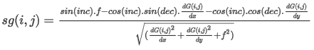
Where:

sg -> shadow grid

i,j -> i^th row & j^th column grid indices

inc -> illumination inclination

dec -> illumination declination

f -> 1/ VerticalScaleFactor

dG(i,j)/dx -> gradient of the i,j grid point in the X directions

dG(i,j)/dy -> gradient of the i,j grid point in the Y directions

HSV

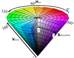The Hue component describes the colour itself in the form of an angle between [0°,360°]. The illustration shows the angular values of the entire colour pallet. For example red is assigned 0° and cyan is at 180°. To abide to the Geosoft colour table format, colour must be represented with a 1 byte integer, thus the 360 range is scaled to a 255 range. When invoked, the Display Grid tool converts it to the right range on the fly. The Saturation component is between 0 & 1, where 0 indicates the absence of colour and 1 its full intensity. In the illustration, it is represented by the radius of the circle.

The Value component spans from 0 to 1, where 0 is the darkest (black - at this point the values of H and S are irrelevant), 1 the brightest. In the illustration, it is represented by the vertical component. The S & V components influence the shading and the contrast, which are controlled by the inclination and declination of the sun angle. To abide to the Geosoft colour table format, both the S & V components are also scaled to [0,255], and the Display Grid tool converts them to the right range on the fly. The colour distribution for a HSV image (1st column of hsvc.tbl) is translated to the 3 RGB components on the fly and scaled for brightness and contrast ( 2nd & 3rd columns of hsvg.tbl) along the sun shadow angle. Unlike the RGB colour distribution option, the HSV tables are not static tables but generated on the fly, and as a result you can not use the Colour tool to modify it.

Crooked Section Grids

Vertically gridded profile data is frequently collected, extracted, or calculated along a line that has a non-straight path; such data is displayed in Oasis montaj using a specially defined grid orientation called "crooked section".

The following is an example of a crooked section grid displayed with a vertical exaggeration in a 3D View:

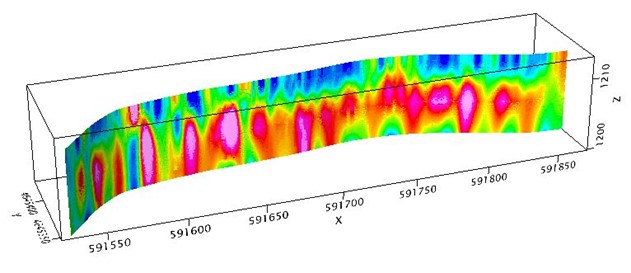
The data grid format used for the crooked section grids is the same as the one used for regular plan and section grids with the “Y” axis (grid columns) corresponding to the elevation and the “X” axis values corresponding to the distance measured along the line.

The information required to specify the grid “trace” is stored as an “orientation” inside the grid projection information (the IPJ class), and consists of locations along the grid trace (line path) as well as the distance recorded at each location:

(x0, y0, d0), (x1, y1, d1), …. (xn-1, yn-1, zn-1)

The number of trace locations does not have to be equal to the number of columns in the grid, nor do the locations need to correspond exactly to data locations; however, in many cases they do, and it is a good practice when defining a crooked section trace to ensure that the first and last points correspond to the first and last data column location in the grid.

Why is the distance along the line specified in addition to the locations?

In many cases, the distance is not simply the incremental straight-line distance between points. The distances correspond directly to the distances as defined in the grid “X” axis direction, and no assumptions are made about the exact path between each location (though for purposes of rendering in the third dimension, a straight-line join between points is assumed). This dependence on “D” instead of “X” and “Y” for grid positions means the path can be "thinned out" without losing the tie of each remaining location to an exact location in the grid.

Rendering a Crooked Section Grid in the Grid View

The simplest view of a crooked section grid is in a grid window, where the grid is viewed “stretched out” with the “distance along the path” as the x-axis value and the elevation as the y-axis. The status bar still displays the correct location on the earth, because the cursor location is reprojected from the crooked section x-axis “distance” to the corresponding (X, Y) position for that distance.

Rendering a Crooked Section Grid into a Section View

To render a crooked section grid onto a section view, the crooked section grid data is projected perpendicularly onto the section. For instance, the section might be defined as the flat plane which intersects the crooked section at its beginning and at its end:

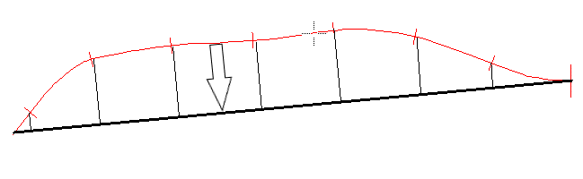
The effect of this projection is to compress the crooked section grid; moreover, the compression is not uniform – the parts of the section, which are angled the most with reference to the view, are compressed the most, while those parts closest to being parallel to the view are almost not at all compressed.

Mathematically, the crooked section (x, y) locations are rotated into the normal section's own coordinate system, where x is along the section, y is the elevation, and z is perpendicular to the section.

For each location Xs in the normal section, the two bracketing path locations are located as: one with Xc lower than or equal to Xs, and one with Xc+1 higher than Xs. Using linear interpolation, the corresponding Dc and Dc+1 are used to determine the D corresponding to the required input location, and given the crooked section origin and grid DX value, the correct column (or columns) of data is determined to project to the required location in the normal section.

Rendering a Crooked Section Grid into a 3D View

To render a crooked section grid into a 3D View, the crooked section is first rendered (as above) onto the vertical plane that joins the beginning and end of the crooked section. Using the same transformation, the “Z” values in the progression – corresponding to the distance that the crooked section deviates from the plane are used to create a relief grid, that, when applied to the projected grid synthesizes the crooked section as if it were a coloured surface in 3D. The process creates two output grids, a “planar” grid and a “relief” grid. Both are rendered at the proper location on a defined plane in the 3D viewer, and as such do not have any type of section orientation. (You can see “planar” in the name of the AGG group of the Group Manager in the 3D viewer.)

Backtracks

Not all crooked section grids can be rendered in 3D using the above method. In addition, you cannot project a crooked section onto all possible flat sections. The reason is "backtracking" in the projected section (the crooked section grids "double-back onto themselves"). Consider projecting the above “E-W” path onto an approximately “N-S” section:

Note that from locations 2 to 3, the projection reverses and overwrites existing values on the projection plane. Any projection needs to be 1-1, so in practice if this situation is encountered, the separation into a projected and relief grid is impossible. You will have the option to plot the grid as a “pixel plot”, where each grid cell is rendered as a single square in 3D. (This eliminates any smoothing effects.)