Numeric Composites

Compositing numeric data takes unevenly-spaced drillhole data and turns it into regularly-spaced data, which is then interpolated. Compositing parameters can be applied to entire drillholes or only within a selected region of the drillhole. For example, you may wish to composite Au values only within a specific lithology.

There are two approaches to compositing numeric data in Leapfrog Geo:

• Composite the drillhole data directly. This creates a new interval table that can be used to build models, and changes made to the table will be reflected in all models based on that table. This process is described below.
• Composites the points used to create an interpolant. This is carried out by generating an interpolant and then setting compositing parameters for the interpolant’s values object. This isolates the effects of the compositing as the compositing settings are only applied to the interpolant.

The rest of this topic describes compositing drillhole data directly. It is divided into:

• Creating a Numeric Composite
• Selecting the Compositing Region
• Compositing Parameters
• Viewing Numeric Composite Statistics

Creating a Numeric Composite

To create a numeric composite, right-click on the Composites folder and select New Numeric Composite. The New Composited Table window will appear:

Set the compositing region and parameters; this is described in detail below. Then click on the Output Columns tab to select from the available columns of numeric data. Click OK to create the table.

Double-clicking on the table displays the data in its columns. Edit the table by right-clicking on it and selecting Edit Composited Table.

Selecting the Compositing Region

Compositing parameters can be applied to entire drillholes or only within a selected region of the drillhole. There are four options for selecting the region in which numeric data will be composited, and each is discussed below.

Compositing in the Entire Drillhole

For this option, Compositing Parameters are applied to all values down the length of drillholes. Select Entire drillhole, then set the compositing parameters.

Compositing in a Subset of Codes

If you wish to select specific category codes in which to composite numeric data, there are two options:

• Subset of codes, grouped
• Subset of codes, ungrouped

The difference between the two is that for the grouped option, the selected codes are combined and the same Compositing Parameters are applied to the grouped intervals:

For the ungrouped option, however, you can set compositing parameters for each code in the selected Base column:

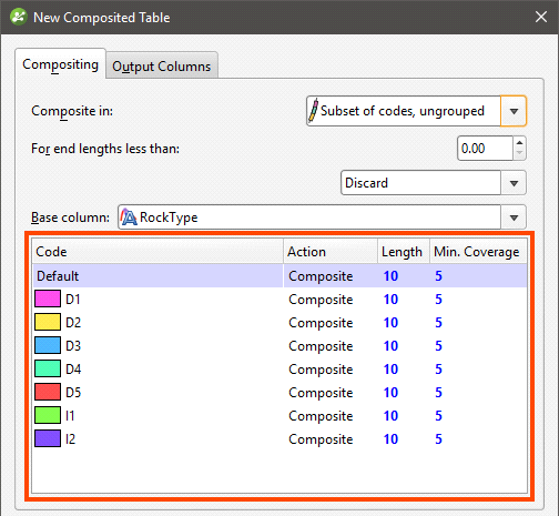
For the Action column, the options are:

• Composite. Numeric data that falls within the selected code will be composited according to the parameters set.
• No compositing. Numeric data is not composited within the selected code. The raw data will be used in creating the new data table.
• Filter out. Numeric data within the selected code will not be included in the new data table.

Compositing in Intervals

For the Intervals from table option, the interval lengths from the Base table are used to determine composite lengths. The value assigned to each interval is the length-weighted average value, and there are no further compositing parameters to set.

Compositing Parameters

When the compositing region is Entire drillhole, Subset of codes, grouped or Subset of codes, ungrouped, the interval lengths are determined by applying three compositing parameters. These parameters are applied as follows:

• The drillholes are divided into intervals wherever numeric data occurs. The Compositing length determines the length of each composite interval, and the Minimum coverage length determines whether or not residual segments (those shorter than the Compositing length) are retained for further processing. Composite lengths are generated from the collar down the drillhole, so any residual segments produced will be at the bottom of the drillhole and where there is data missing down the length of the drillhole. How residual segments are handled is described below.

• The For end lengths less than parameter is applied to determine what happens to the residual segments that may result from applying the Compositing length and Minimum coverage parameters. The three possibilities are Discard, Add to Previous Interval and Distribute Equally.
• Composite values are calculated for each composite interval. This is simply the length-weighted average of all numeric drillhole data that falls within the composite interval.
• Composite points are generated at the centre of each composite interval from the composite values.

Discard

With the Discard option, residual segments that meet or exceed the Minimum coverage length are retained; those shorter are discarded.

For example, consider two drillholes. A is 49 metres long and B is 44 metres long. The Compositing length is set to 10 and the For end lengths less than length is set to 5. There will be a residual segment 9 metres long for Drillhole A and one 4 metres long for Drillhole B. Drillhole A’s residual segment will be retained as a segment, whereas Drillhole B’s residual segment will be discarded. This results in:

• Drillhole A: 10m, 10m, 10m, 10m, 9m (residual length > Minimum coverage length so the 9m segment is kept)
• Drillhole B: 10m, 10m, 10m, 10m (residual length < Minimum coverage length so the 4m segment is discarded)

Add to Previous Interval

With the Add to previous interval option, the Minimum coverage length is automatically set to zero. Residual segments longer than the For end lengths less than value are retained as separate segments; those shorter are added to the previous interval.

For our two drillholes, when the Compositing length is 10, there will be a residual segment 9 metres long for Drillhole A and one 4 metres long for Drillhole B. When For end lengths less than is set to 5, Drillhole A’s residual segment will be retained as a segment, whereas Drillhole B’s residual segment will be added to the previous interval. This results in:

• Drillhole A: 10m, 10m, 10m, 10m, 9m (residual length > For end lengths less than length so the 9m length is kept as a separate segment)
• Drillhole B: 10m, 10m, 10m, 14m (residual length < For end lengths less than length so the 4m segment is added to the previous interval)

Distribute Equally

With the Distribute equally throughout drillhole option, the Minimum coverage parameter is automatically set to zero. Residual segments longer than the For end lengths less than value are retained as separate segments; those shorter will have their length distributed among the other intervals.

For our two drillholes, Drillhole A’s residual segment will be retained as an individual segment, whereas Drillhole B’s residual segment will have its length distributed among the rest of the intervals. The segments for each composited drillhole will be:

• Drillhole A: 10m, 10m, 10m, 10m, 9m (residual length > For end lengths less than length so the 9m segment is kept as a separate segment)
• Drillhole B: 11m, 11m, 11m, 11m (residual length < For end lengths less than length so the 4m length is distributed among the other intervals)

Viewing Numeric Composite Statistics

Once you have created a composited table, you can view statistics on the table or for each individual column in the table.

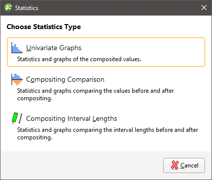
To view statistics for the table, right-click on it and select Statistics.

See the Analysing Data topic for more information on each option:

• Table of Statistics
• Scatter Plots
• Q-Q Plots
• Box Plots

The Interval Length Statistics graph is a univariate graph, so for more information on the options available, see Univariate Graphs in the Analysing Data topic.

Right-click on the table columns and select Statistics to view information about the composited values.

The first option displays statistics on the composited values; see Univariate Graphs in the Analysing Data topic for more information. The other two options display statistics comparing data before and after compositing.

Compositing Comparison

The double histogram, one displaying the distribution of the raw data and one displaying the distribution of the composited data, enables comparison of the two distributions of the same element before and after the compositing transformation. Impacts on the symmetry of distributions will be evident.

In the Histogram settings, Bin width changes the size of the histogram bins used in the plot.Percentage is used to change the Y-axis scale from a length-weighted scale to a percentage scale.

The Box Plot options control the appearance of the box plot drawn under the primary chart. The whiskers extend out to lines that mark the extents you select, which can be the Minimum/maximum, the Inner fence or the Outer fence. Inner and outer values are defined as being 1.5 times the interquartile range and 3 times the interquartile range respectively.

The Limits fields control the ranges for the X-axis and Y-axis. Select Automatic X axis limits and/or Automatic Y axis limits to get the full range required for the chart display. Untick these and manually adjust the X limits and/or Y limits to constrain the chart to a particular region of interest. This can effectively be used to zoom the chart.

The bottom left corner of the chart displays a table with a comprehensive set of statistical measures for the data set.

Compositing Interval Lengths

This graph shows a double histogram of distributions of the interval lengths before and after compositing.

In the Histogram settings, Bin width changes the size of the histogram bins used in the plot.Percentage is used to change the Y-axis scale from a length-weighted scale to a percentage scale.

The Box Plot options control the appearance of the box plot drawn under the primary chart. The whiskers extend out to lines that mark the extents you select, which can be the Minimum/maximum, the Inner fence or the Outer fence. Inner and outer values are defined as being 1.5 times the interquartile range and 3 times the interquartile range respectively.

The Limits fields control the ranges for the X-axis and Y-axis. Select Automatic X axis limits and/or Automatic Y axis limits to get the full range required for the chart display. Untick these and manually adjust the X limits and/or Y limits to constrain the chart to a particular region of interest. This can effectively be used to zoom the chart.

The bottom left corner of the chart displays a table with a comprehensive set of statistical measures for the data set.

 

Got a question? Visit the My Leapfrog forums at https://forum.leapfrog3d.com/c/open-forum or technical support at http://www.leapfrog3d.com/contact/support