Variogram Models

Variography is the analysis of spatial variability of grade within a region. Some deposit types, e.g. gold, have high spatial variability between samples, whereas others, e.g. iron, have relatively low spatial variability between samples. Understanding how sample grades relate to each other in space is a vital step in informing grades in a block model. A variogram is used to quantify this spatial variability between samples.

In estimation, the variogram is used for:

• Selecting appropriate sample weighting in Kriging and RBF estimators to produce the best possible estimate at a given location
• Calculating the estimators’ associated quality and diagnostic statistics

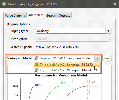
In Leapfrog Geo domained estimations, variograms are created and modified using the Spatial Models folder. As described in Domained Estimations, a default variogram is added to the Spatial Models folder when a domained estimation is created. You can edit this default variogram model or create new ones, as required, for your domained estimation.

• To edit an existing variogram model, double-click on it () in the project tree.
• To create a new one, right-click on the Spatial Models folder and select New Variogram Model.

You can define as many variograms as you wish; when you define an estimator that uses a variogram model, you can select from those available in the domained estimation’s Spatial Models folder:

Working with variograms is an iterative process. The rest of this topic provides an overview of the Variogram Model window and describes how to use the different tools available for working with variograms. This topic is divided into:

• The Variogram Model Window
• The Ellipsoid Widget
• Model Controls
• Experimental Controls

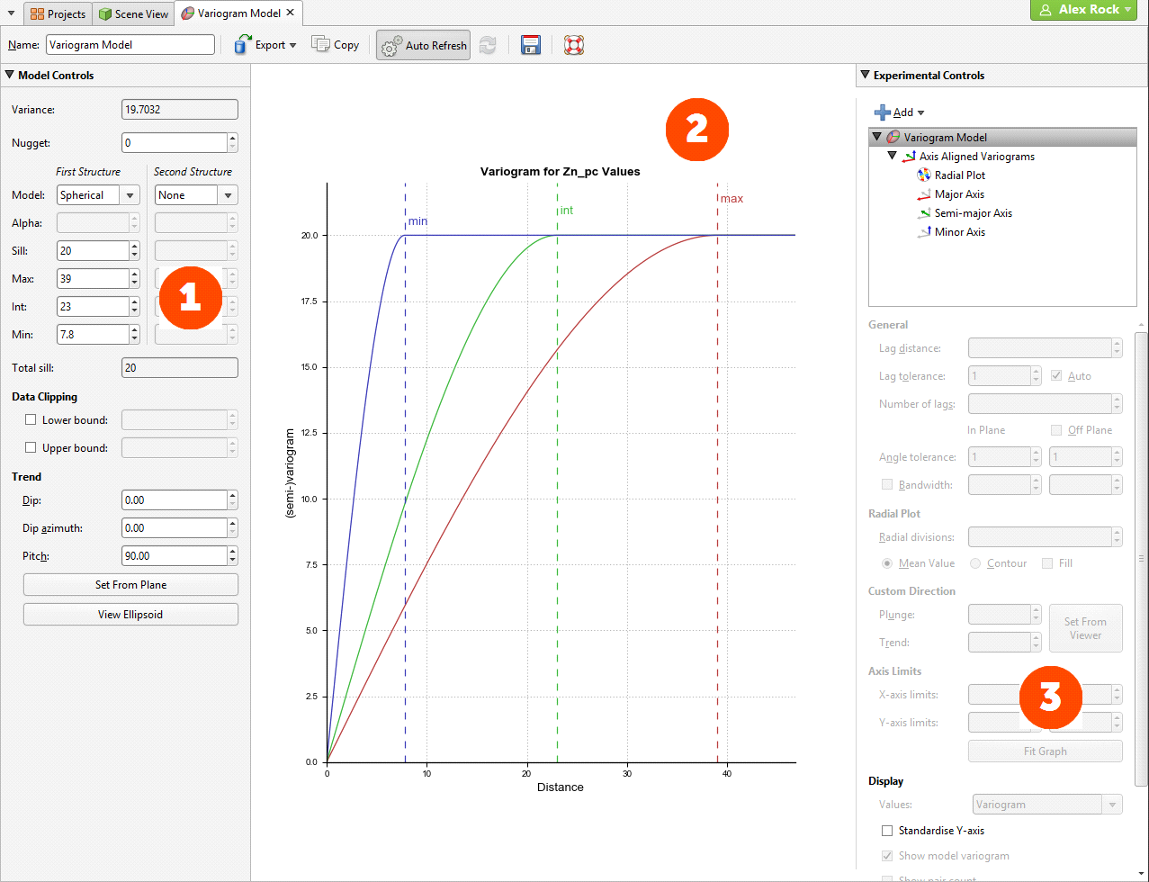
The Variogram Model Window

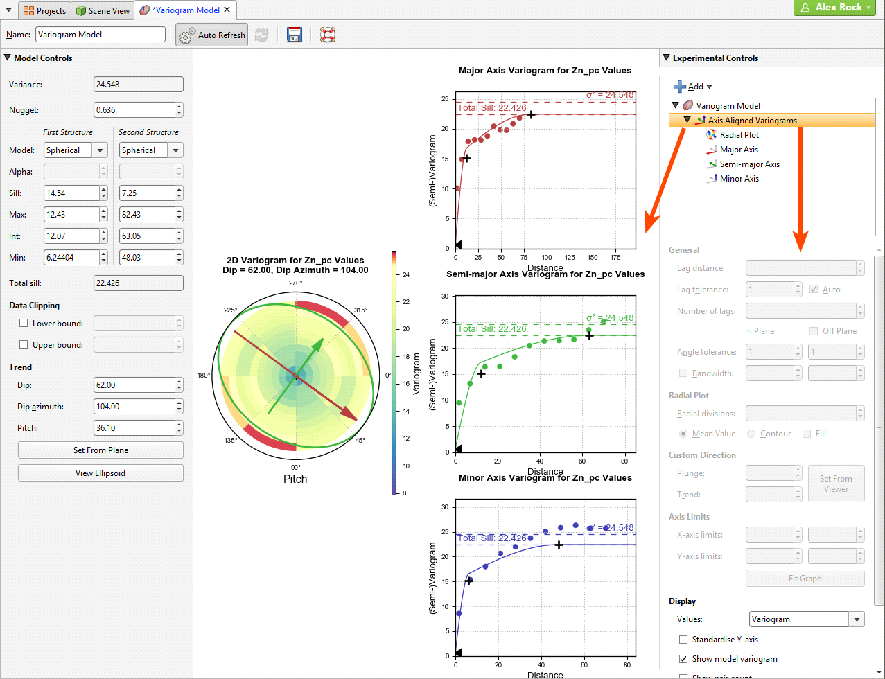
The Variogram Model window is divided into three parts:

	Model controls for adjusting the variogram model type, trend and orientation. See Model Controls below. To make more room to view the selected variogram, this panel can be hidden by clicking the triangle next to the Model Controls label. Clicking it again will reveal the panel.
	Graphs plotting the selected variogram
	Experimental controls for verifying the theoretical variogram model. See Experimental Controls below. To make more room to view the selected variogram, this panel can be hidden by clicking the triangle next to the Experimental Controls label. Clicking it again will reveal the panel.

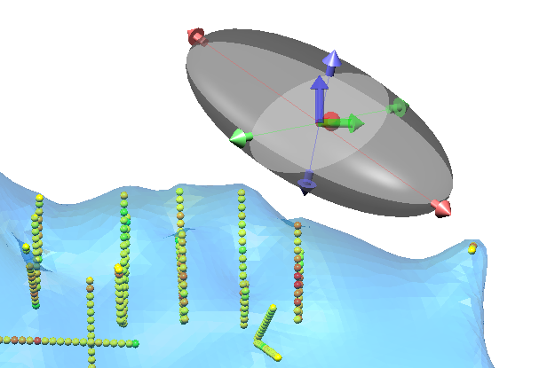
When you edit a variogram model in the Variogram Model window, an ellipsoid widget is automatically added to the scene. The ellipsoid widget helps you to visualise the variogram in 3D, which is useful in setting variogram rotation and ranges and in defining search neighbourhoods. See The Ellipsoid Widget below for more information.

If the Variogram Model window is docked as a tab, you can tear the window off. As a separate window, you can move and resize the window so you can see the ellipsoid change in the 3D scene while you make adjustments to the model settings. The detached window can be docked again by dragging the tab back alongside the other tabs, as described in Organising Your Workspace.

There are two ways to save the graph for use in another application:

• Click the Export graph button () to export the graph as a PDF, PNG or SVG file.
• Click the Copy graph button () to copy the graph to the clipboard. You can then paste it into another application.

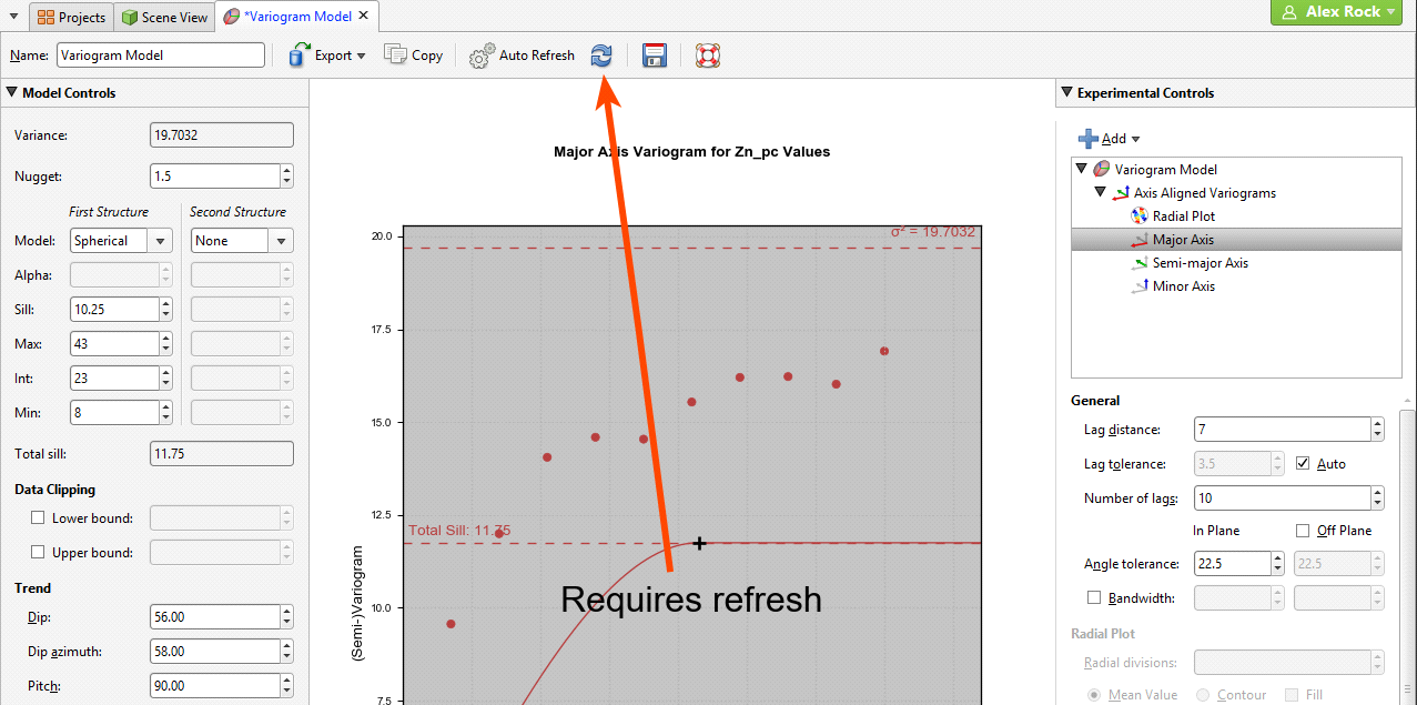
There are two buttons for refreshing the graphs when changes are made:

• When Auto Refresh is enabled, recalculations will be carried out each time you change a variogram value. This can produce a brief lag.
• When auto refresh is disabled, you can click the Refresh button () whenever you want the graphs to be updated. This is the best option to use when working with a large dataset.

If auto refresh is disabled and values have been changed without the graphs being updated, the chart will turn grey and a reminder will be displayed over it:

The Ellipsoid Widget

With variograms, you can display the ellipsoid in the 3D scene in order to:

• Visualise the variogram model in the scene
• Set variogram rotation and ranges
• Define search neighbourhoods

The ellipsoid has handles for changing the orientation, and if you have the Variogram Model window displayed alongside the scene window, you will see the settings in the Variogram Model window change as you change the ellipsoid in the scene.

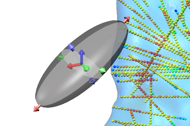
Click on the widget to toggle between control modes. Each mode offers different handles for directly manipulating the ellipsoid widget. When the arrows on the edge of the widget are yellow, blue and red, the handles adjust the ellipsoid trend.

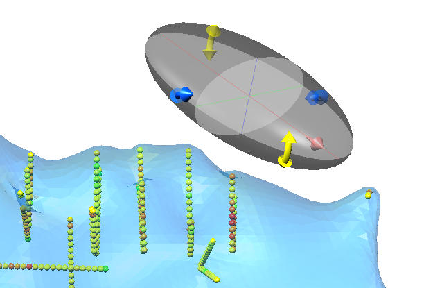
Drag a yellow arrow handle to adjust the Dip, blue to adjust the Dip Azimuth and red to adjust the Pitch.

When the arrows on the edge of the widget are red, green and blue, the handles adjust the ellipsoid ranges.

Drag a red arrow handle to adjust the Max axis range, green to adjust the Int range and blue to adjust the Min range.

In the properties panel for the variogram model trend, settings control the Centre Point of the ellipsoid widget. The X, Y and Z position can be specified directly.

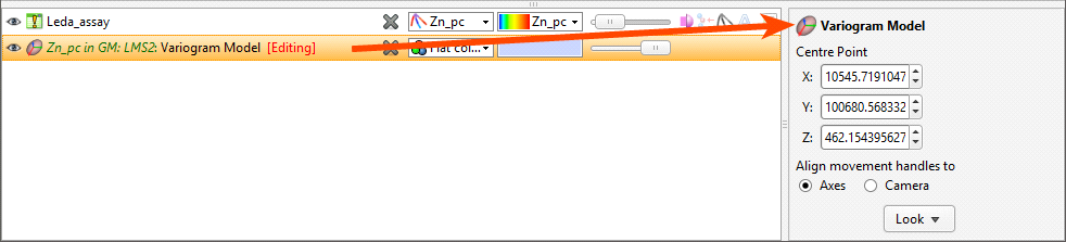
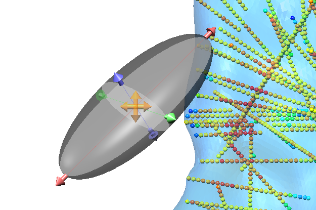
It is also possible to drag the ellipsoid to a different location. If the ellipsoid does not have arrows in the centre, click the ellipsoid so that the movement arrows appear. You can click the ellipsoid again to turn them off. Click and drag the movement arrows to reposition the ellipsoid widget in the screen. Two movement modes are possible: In the properties panel, you can choose to Align movement handles to the Axes or the Camera. When Align movement handles to is set to Axes, the handles in the centre of the widget are red, green and blue. Click on one of these arrows and you will be able to drag the widget back and forth along the orientation of your selected axis:

Don’t confuse the red, green and blue centre point arrows with the red, green and blue axis adjustment arrows that may appear on the edge of the widget.

When Align movement handles to is set to Camera, the handles in the centre of the widget are orange. Click on these arrows and you can drag the widget left-and-right and up-and-down in the viewing plane.

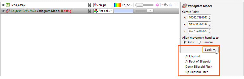
The Look button provides options for quickly changing the camera viewpoint.

To aid in the visualisation of the ellipsoid, the major-intermediate axial plane and the intermediate-minor axial plane have been drawn and shaded. The major, intermediate and minor axes are also drawn as red, green and blue lines respectively. This assists in visualising the orientation and shape of the ellipsoid. In some views, the planes are exchanged for alternate planes, such as when displaying octant search sectors.

Model Controls

The Model Controls adjust the theoretical variogram model type, trend and orientation. The graph in the middle of the window will change as model parameters are adjusted. The ellipsoid in the scene will also reflect the changes you make to the Model Controls.

Variance is calculated automatically from the data and shows the magnitude of the variance for the dataset.

Multi-structured variogram models are supported, with provision for nugget plus two additional structures.

The Nugget represents a local anomaly in values, one that is substantially different from what would be predicted at that point based on the surrounding data. Increasing the value of Nugget effectively places more emphasis on the average values of surrounding samples and less on the actual data point and can be used to reduce noise caused by inaccurately measured samples.

Each additional structure has settings for the Model, Alpha (if the model is spheroidal), the component Sill, and the Max, Int and Min ellipsoid ranges.

Linear, Spherical and Spheroidal Model Options

Model provides three options: Linear, Spherical and Spheroidal.

Linear is a general-purpose multi-scale option suited to sparsely and/or irregularly sampled data. Spherical and Spheroidal are suitable for modelling most metallic ores, where there is a finite range beyond which the influence of the data should fall to zero. A Spherical model has a range beyond which the value is the constant sill. A Spheroidal model flattens out when the distance from the sample data point is greater than the range. At the range, the function value is 96% of the sill with no nugget, and beyond the range the function asymptotically approaches the sill. Each axis of the variogram ellipsoid has its own range, adjusted using Max, Int and Min. The ranges are colour-coded in the variogram model plot.

Alpha is only available when the Model is Spheroidal. The Alpha constant determines how steeply the interpolant rises towards the Sill. A low Alpha value will produce a variogram that rises more steeply than a high Alpha value. A high Alpha value gives points at intermediate distances more weighting, compared to lower Alpha values. An Alpha of 9 provides the curve that is closest in shape to a spherical variogram. In ideal situations, it would probably be the first choice; however, high Alpha values require more computation and processing time, as more complex approximation calculations are required. A smaller value for Alpha will result in shorter times to evaluate the variogram.

Sill defines the upper limit of the model, the distance where there ceases to be any correlation between values. A spherical variogram reaches the Sill at the range and stays there for increasing distances beyond the range. A spheroidal variogram approaches the Sill near the range, and approaches it asymptotically for increasing distances beyond the range. The distinction is insignificant. A linear model has no Sill in the traditional sense, but along with the ellipsoid ranges, Sill sets the slope of the model. The two parameters sill and range are used instead of a single gradient parameter to permit switching between linear, spherical and spheroidal interpolant functions without also manipulating these settings. Each structure has a component Sill.

The Total Sill is displayed below the First Structure and Second Structure settings.

Data Clipping

Data Clipping fields cap the Lower bound and Upper bound for the data as specified. This is not a filter that discards these points, but values below or above the caps are treated as if the value was the lower or upper bound.

Trend Directions

The Trend fields set the orientation of the variogram ellipsoid. Adjust the ellipsoid axes orientation using the Dip, Dip Azimuth and Pitch fields.

The Set From Plane button sets the trend orientation of the model ellipsoid based upon the current settings of the moving plane

The View Ellipsoid button adds a 3D ellipsoid widget visualisation to the scene.

Experimental Controls

A theoretical variogram model can be verified through the use of the experimental variography tools that use data acquired in the drilling process. Use these to find the directions of maximum, intermediate and minimum continuity.

The variogram displayed in the chart is selected from the variograms listed in the Experimental Controls panel.

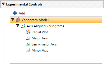
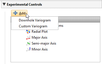
By default, there is a set of Axis Aligned Variograms. Use the Add button to add experimental variograms. You can add one Downhole Variogram and any number of Custom Variograms.

Click on one of these experimental variograms to select it and display its parameters. The graph in the middle of the Variogram Model window will change to match this selection. For example, here the graph and settings for the Axis Aligned Variograms are displayed:

Selecting the Semi-major Axis variogram changes the chart and settings displayed:

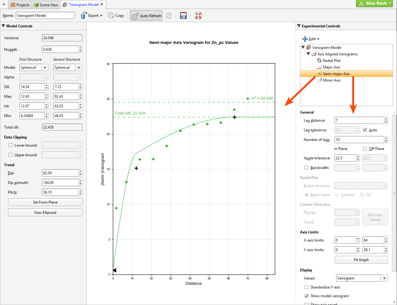
Adjust the model variogram parameters to see the effect different parameters have when applied to the actual data.

Experimental Variogram Parameters

The settings under Experimental Controls define the search space, define the orientation for custom variograms and change how the variograms are displayed. Some parameters are only available for some variogram types; these are discussed in later sections on each variogram type.

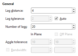
Defining the Search Space

The first set of parameters controls the search space.

• Lag distance controls the size of the lag bins. The first bin will be half the size of the Lag distance. Experimental variograms generally measure lags as distances along a direction vector, though downhole variograms measure lags as distances along the drillholes.
• Lag tolerance allows for the reality that data pairs are rarely the same distance apart. The data is scanned and pairs are assembled after applying a Lag tolerance to the Lag distance. If the Lag tolerance Auto box is ticked, Leapfrog Geo defaults to using a Lag tolerance of half the Lag distance. Controlling the Lag tolerance explicitly allows you to test the sensitivity of the variogram. Typically, a larger value will be used for sparse datasets and a smaller value for dense datasets.

• Number of lags constrains the number of lag bins in the search space.
• The In Plane and Off PlaneAngle tolerance and Bandwidth settings define the search shape, and the effects of these settings are discussed in more detail below.

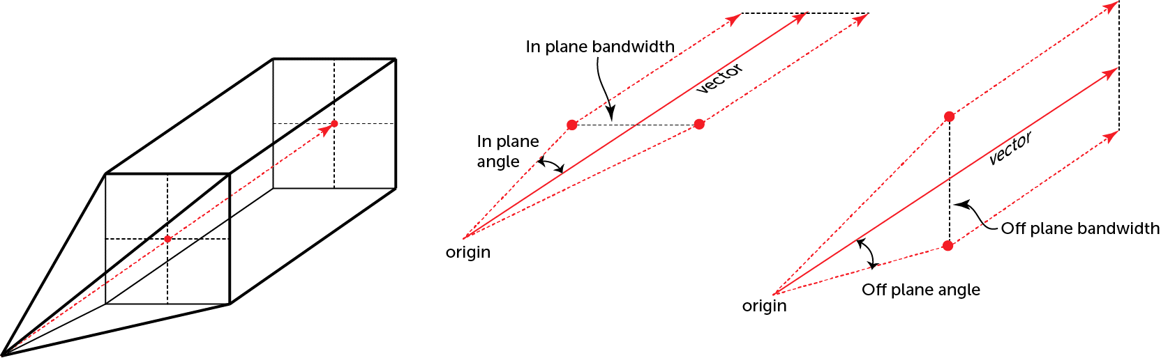
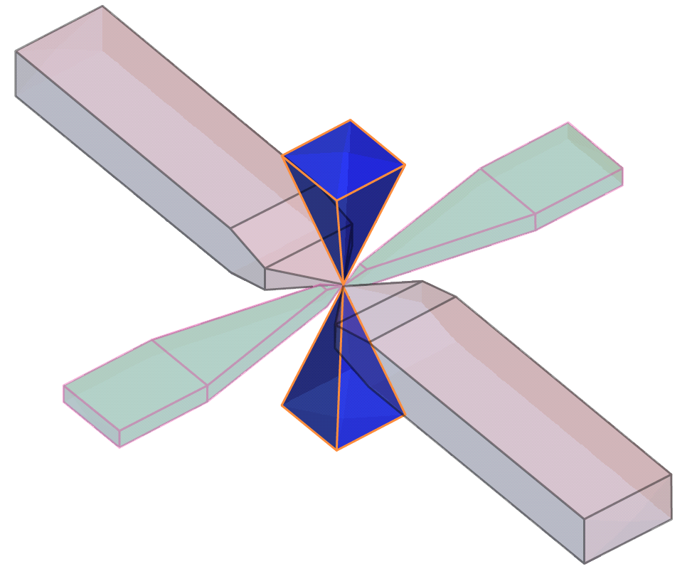
The search shape usually approximates a right rectangular pyramid on a rectangular parallelepiped. The pyramid and parallelepiped will be square if the In Plane Angle tolerance and Bandwidth are used without defining Off Plane values. Using the Off Plane Angle tolerance and Bandwidth fields will make the shape rectangular. The plane being referred to is the major-intermediate axis plane of the variogram ellipsoid, the same plane used for the radial plot. The Angle tolerance is the angle either side of a direction vector from the data point origin. Once the sides of the pyramid defined by the angle tolerances extend out to the limits specified by the Bandwidth, the search neighbourhood is constrained to the bandwidth dimensions.

The search shape becomes a more complex “carpenter’s pencil” shape when a wide In Plane angle and a narrow Bandwidth are defined along with a narrow Off Plane angle and a wide Bandwidth, or vice versa. This rendering should assist in visualising the shape; the major axis is shown in red, the semi-major axis is shown in green, and the orthogonal minor axis in a transparent blue:

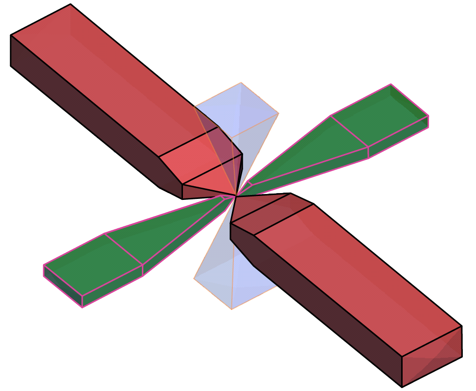
Note that although not shown here, the outer ends of the search shapes are not flat, but rounded, being defined by the surface of a sphere with a radius of the maximum distance defined by the number of lags and their size.

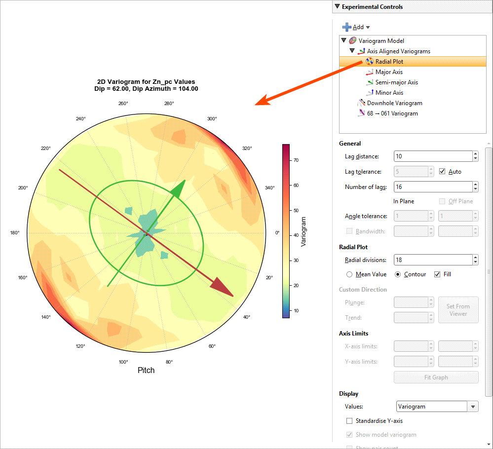
Radial Plot Parameters

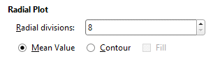
Radial Plot has parameters specifically for the radial plots in Axis Aligned Variograms.

Increasing the Radial divisions increases the resolution of the radial plot, with each block in the radial plot covering a smaller arc of the compass. Using a high value will increase the resolution used to improve precision, but this carries a calculation time cost. Using a smaller number will be faster, but will be less useful for observing directions of continuity. The default value of 8 is fast, but you may want to turn off Auto Refresh Graphs and increase the number of Radial divisions before clicking Refresh graphs.

Mean Value will display radial plot bins coloured to indicate the mean value for each bin. Contour will display a plot showing lines of equal value. Fill shades the chart between the contour lines.

Orienting Custom Variograms

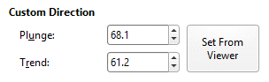
The Custom direction fields are for Custom Variograms that use the Plunge to Trend settings to orient the variogram trend. They can easily be set by orienting the scene view and then clicking the Set From Viewer button, which sets the plunge and trend to that of the scene view.

Changing Variogram Display

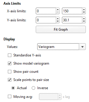
The Axis Limits settings control the chart scaling.

X axis limits and Y axis limits control the ranges for the X-axis and Y-axis and can effectively be used to zoom the chart. You can directly control these by manipulating the axes with your mouse. Click and drag an axis to increase or decrease the maximum limit of the axis. Right-click and drag an axis to reposition the axis so the minimum value on the axis is not zero. Double-click the axis to reset the axis minimum and maximum range to the default values.

The Display settings change how the variogram is displayed:

• Values offers a variety of options to plot on the chart: Variogram, Correlogram, Covariance, Relative Variogram and Pair-wise Variogram.
• Standardise Y-axis changes the Y-axis scale to a standardised scale, normalised by the global variance of the base data, respecting any clipping specified. Scaled variograms can be used to estimate different elements in the same domain or to apply a detailed variography model in one domain to an adjacent domain.
• Show model variogram plots the variogram on the chart.
• Show pair count annotates the chart with the count of data point pairs.
• Tick the Scale points to pair size checkbox and the chart will display the plotted points with dots that scale to the size of the pair count. Choose Actual so the dots represent the pair size proportionally and Inverse to see larger dots for lower pair counts.

• Tick Moving avg for a rolling mean variogram value, drawn on the variogram plots in orange. Next to it, select a value for the window size relative to the Lag distance.The window size will be the given number times the lag distance. This window, centred on x, will be used to plot y, the average of all the variogram values falling inside the window.

The Downhole Variogram

The Downhole Variogram can be used to better define the nugget. It looks only looks at pairs of samples on the same drillhole and uses the differences in depths to calculate the lag value.

As it isn’t associated with a specific direction, the Angle tolerance parameter is not available for the Downhole Variogram.

The Downhole Variogram chart does not plot the model variogram line; instead it shows a dotted horizontal line indicating the Sill:

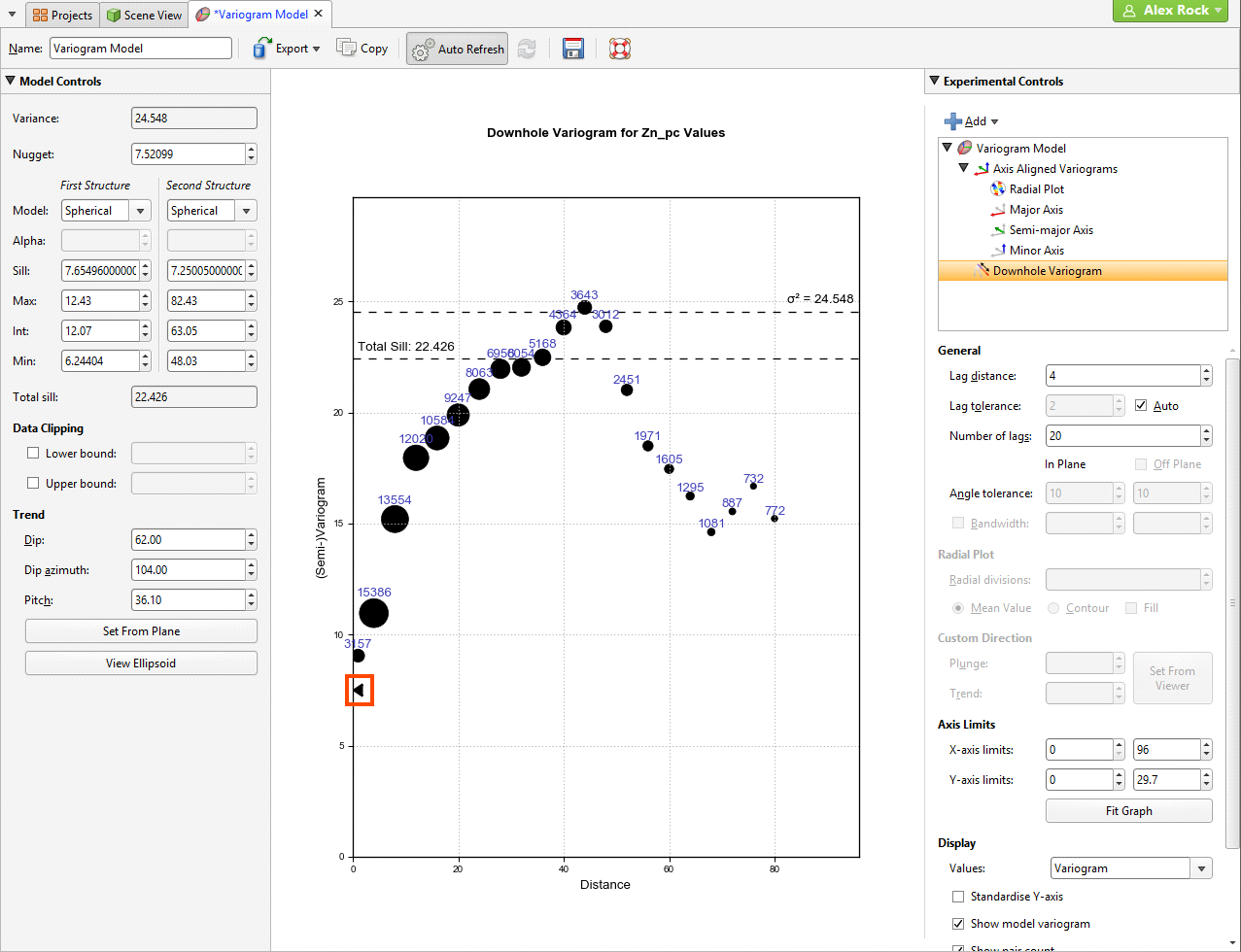
A triangular dragger handle next to the chart’s Y-axis can be used to adjust the Nugget value in the Model Controls part of the window. As the downhole values are nearly continuous, an accurate estimate can be made for the nugget effect for this direction.

Axis Aligned Variograms

The Axis Aligned Variograms are useful for determining the direction of maximum, intermediate and minimum continuity. When you select the Axis Aligned Variograms option, all four variograms are displayed in the chart:

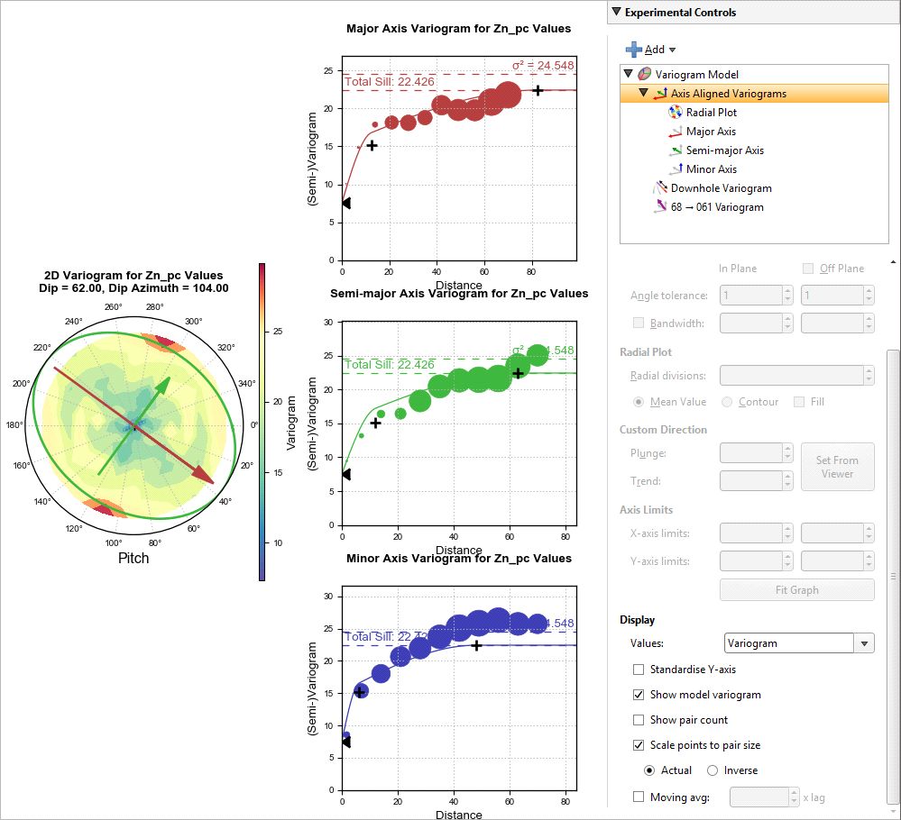
The radial plot and each of the axes variograms can be viewed in greater detail by clicking on them in the variogram tree:

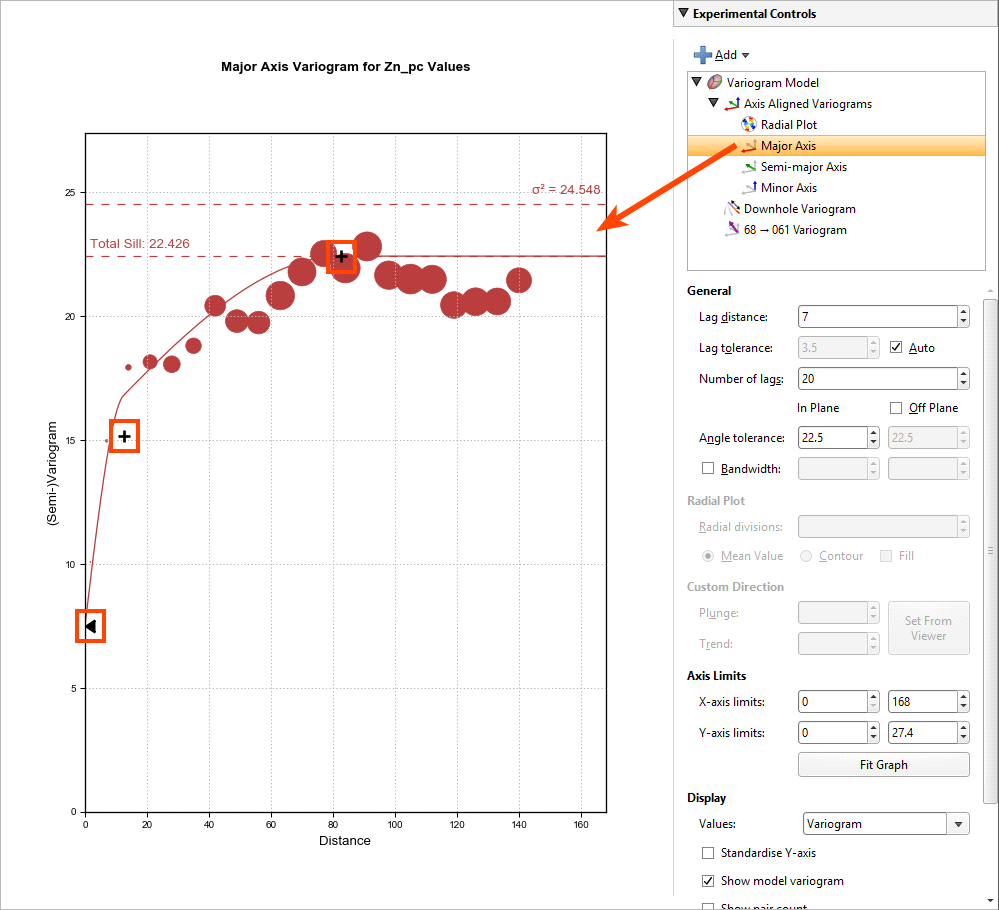
In the axes variogram plots, you can click-and-drag the plus-shaped dragger handle to adjust the range and the sill. A triangular dragger handle adjusts the nugget. A solid line shows the model variogram, and dotted horizontal lines show the sill and variance.

In the radial plot, you can click-and-drag the axes arrows to adjust the pitch setting, between the values 0 and 180 degrees. Each bin in the mean value radial plot shows the mean semi-variogram value for pairs of points binned by direction and distance. When the contour plot is selected, lines follow the points of equal value.

Custom Variograms

Any number of custom variograms can be created. These are useful when validating a model, for checking the variogram directions other than the axis-aligned directions. The Plunge to Trend settings determine the direction of the experimental variogram, and these are set independently of the Dip, Dip Azimuth and Pitch settings used by the other experimental variograms. The Plunge to Trend settings can be quickly set by orienting the scene and then clicking the Set From Viewer button in the Variogram Model window. This copies the current scene azimuth and plunge settings into the fields for the custom variogram.

When selected, the custom variogram shows a semi-variogram plot, with the model variogram plotted:

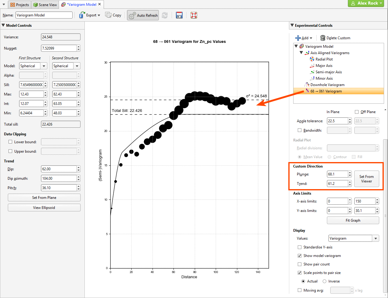
There are no handles on this chart. Dotted horizontal lines indicate the sill and variance.

 

Got a question? Visit the My Leapfrog forums at https://forum.leapfrog3d.com/c/open-forum or technical support at http://www.leapfrog3d.com/contact/support