Trends and Anisotropy
A point source of light radiates in all directions equally, and the intensity of that radiated light decreases at a rate equal to the inverse of the square of the distance from the source. This radiation is isotropic, and in many fields isotropic behaviour can be assumed when making measurements. Geologists are well aware that, in their field, this cannot be assumed. Because of the processes involved in rock and strata formation involving sedimentation, compression and igneous flows, measurements can demonstrate strong trends in one particular direction or plane, but weak trends in an orthogonal direction. Leapfrog provides tools to account for this anisotropy when modelling, including:
Global Trends
The most basic anisotropy tool is the global trend. As the name suggests, this applies the anisotropic trend globally. It is suitable for use in situations where the underlying geology suggests that the anisotropy is planar and continuous over a large area. The global trend sets a constant trend that will favour grade continuity in one direction. When calculating interpolants and modelling, the application of this global trend will reflect the favouring of the trend direction.
Where an object includes a Trend tab in its settings, you can directly specify the Dip, Dip Azimuth and Pitch directions, as well as the Maximum, Intermed and Minimum ellipsoid ratios.
The global trend is expressed in the form of ratios in three orthogonal directions, described as the major (“Maximum”), semi-major (“Intermed”) and minor (“Minimum”) axes of an ellipsoid. When the same value is used for each axis, the ellipsoid is spherical and the global trend is isotropic. Reducing the ratio in the minor axis direction relative to the major and semi-major axes produces an oblate discus-shaped anisotropic trend that de-emphasises the minor axis direction. This sort of global trend is typical for modelling structures that have undergone compression.
Increasing the ratio value in the major axis direction, while having a lower ratio for the semi-major axis and smaller still for the minor axis, further emphasises the trend in the Maximum direction. This sort of global trend is typical for modelling structures formed from flows. When the geology is modelled, the Maximum direction of the trend is favoured over the other directions, and the Minimum direction is de-emphasised.
When the semi-major and minor axes have the same value and the major axis is larger, this emphasises the trend in only in the Maximum direction. This results in a prolate cigar-shaped anisotropic trend.
Leapfrog does not enforce that the ratios for the global trend axes are such that the values for Maximum > Intermediate > Minimum. As such, it is possible to create an ellipsoid that has a trend strongest in, say, the Minimum direction. This should be avoided as it will likely produce confusion, especially for others endeavouring to understand the geology modelled in the project.
The global trend ellipsoid can be oriented in any direction other than the x, y and z axes of the model by rotating it using Dip, Dip Azimuth and Pitch controls.
You can use the View Plane button to add a moving plane to the scene and use the handles on the moving plane to adjust the Dip, Dip Azimuth and Pitch which will be updated when the Set From Plane button is clicked. The moving plane indicates the orientation of the major-semimajor axis of the trend ellipsoid, with the Maximum trend direction in the direction of the green Pitch arrow. Ellipsoid ratios cannot be set from the moving plane.
The Ellipsoid Ratios determine the relative shape and strength of the ellipsoids in the scene, where:
- The Maximum value is the relative strength in the direction of the green line on the moving plane.
- The Intermed. value is the relative strength in the direction perpendicular to the green line on the moving plane.
- The Minimum value is the relative strength in the direction orthogonal to the plane.
Often the easiest way to apply a trend is to click on the Draw plane line button (![]() ) and draw a plane line in the scene in the direction in which you wish to adjust the surface. You may need to rotate the scene to see the plane properly. Once you have adjusted the plane to represent the trend you wish to use, click the Set From Plane button to copy the moving plane settings.
) and draw a plane line in the scene in the direction in which you wish to adjust the surface. You may need to rotate the scene to see the plane properly. Once you have adjusted the plane to represent the trend you wish to use, click the Set From Plane button to copy the moving plane settings.
The Set to list contains a number of different options Leapfrog Geo has generated based on the data used in the project. Isotropic is the default option used when the surface was created. Settings made to other surfaces in the project will also be listed, which makes it easy to apply the same settings to many surfaces.
Anisotropic or Ellipsoidal Distance
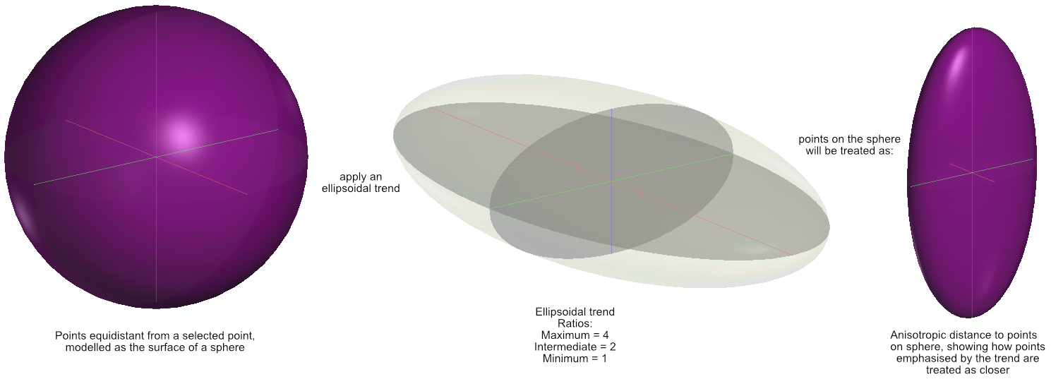
When a trend is applied during modelling, distances between points are scaled proportionally to the ellipsoidal trend, creating a concept called the anisotropic distance or ellipsoidal distance. When interpolating to calculate a value at a specific point, measured data points closer to that point will have more influence in the interpolation calculation. When a trend is applied, the anisotropic distance is used instead of the actual distance. In the trend's Maximum direction we want the measured data points to have more influence, so the anisotropic distance is smaller than the actual distance. We divide the actual distance by the Maximum axis ratio, so if the ellipsoid Maximum ratio is 4, the anisotropic distance to a point in the maximum direction is ¼ the actual distance, significantly increasing the influence of a measured point in that direction. If the Intermediate ratio is 2, the anisotropic distance to a point in the intermediate direction is ½ the actual distance, again increasing the influence of a measured point in that direction, though not as significantly as in the Maximum direction. Consider this diagram demonstrating how points equidistant from a central point are treated when an anisotropic trend is applied, with the ratios Maximum = 4, Intermediate = 2 and Minimum = 1.
It may be useful to think of the ellipsoidal trend as warping spacetime, making the apparent anisotropic distance or ellipsoidal distance shorter in emphasised directions. Still, it is not normally necessary to envisage things by anisotropic distances. More intuitively, interpolated surfaces modelled using trends clearly demonstrate the emphasis indicated by the trend ellipsoid proportions and orientation.
When you have the Leapfrog Edge extension, the trend can also be visualised in the scene as an ellipsoid. For more information, see The Ellipsoid Widget.
Where the underlying geology shows that it cannot be assumed that the anisotropy is planar and continuous over a large area, Leapfrog provides additional tools.
Structural Trends
When there is a gradual shift in the direction of the grade continuity, perhaps due to flows, a global trend will not suffice to model the geology. In this case, Leapfrog's structural trend tool is more appropriate. A structural trend localises trend modelling to indicate changes in direction of continuity. A selected surface or structural data is used as an indicator to locally align the trend direction. The result is that for any given point of interest, the trend orientation is specific and appropriate to that location.
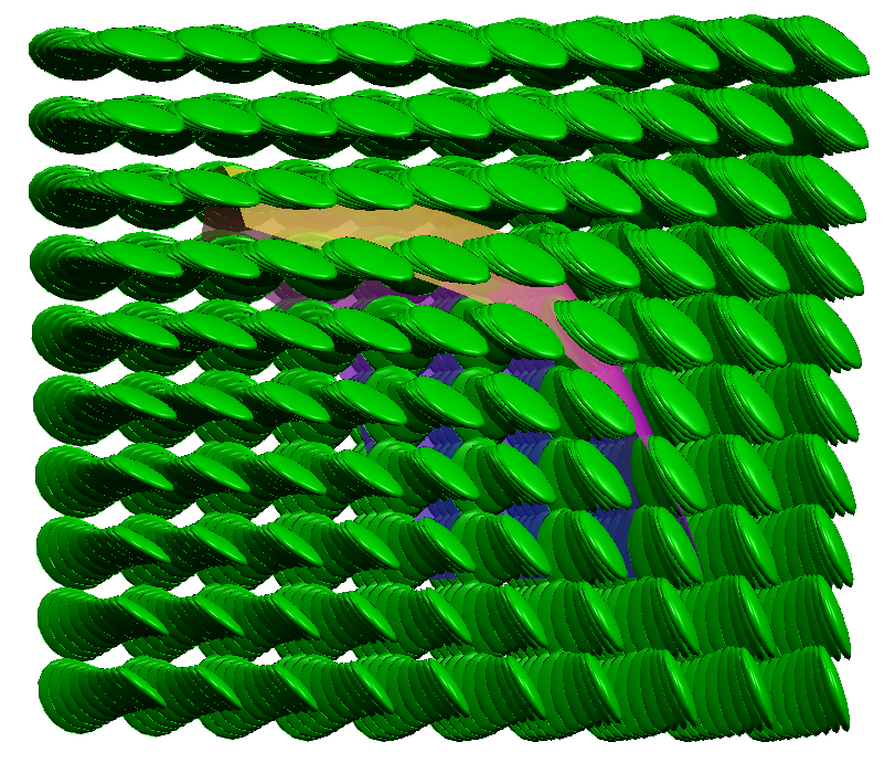
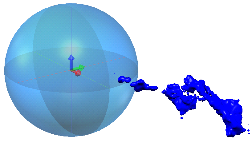
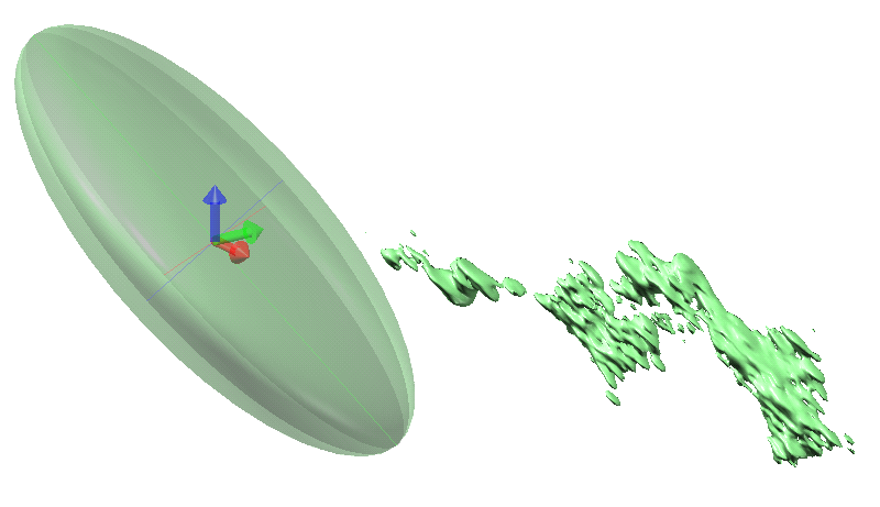
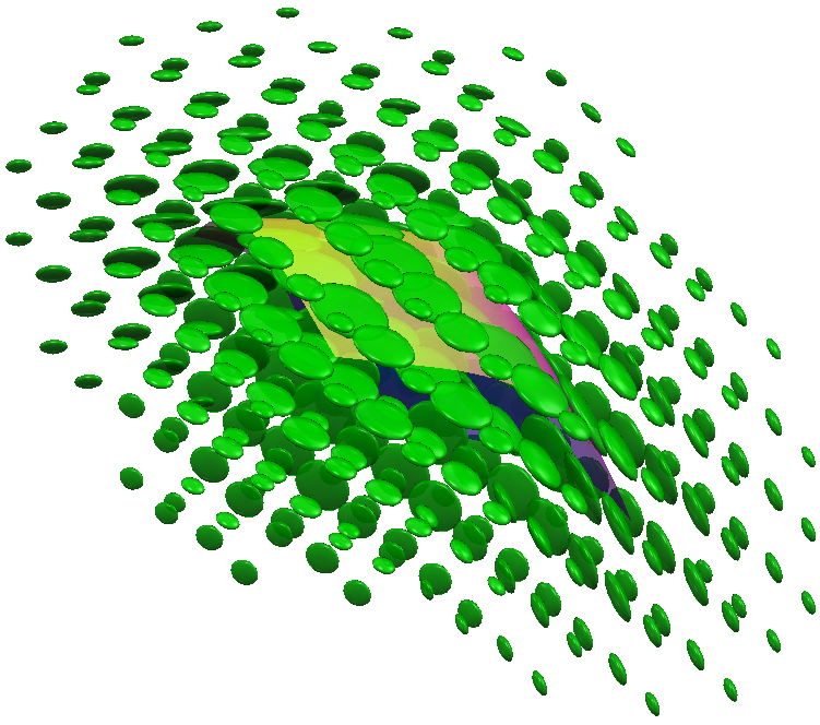
When displayed in the scene, the structural trend is rendered as a grid of oblate ellipsoids. The grid has regular 10x10x10 spacing which enclose the extents of the structural trend's inputs. The orientation of the disk gives the direction of the anisotropy. The size of a disk is proportional to the anisotropy strength. Where there are no disks (or the size is very small) the trend is isotropic.
Note that when a structural trend is used in an interpolation, the locations of the depicted ellipsoids are not the only locations influenced by the structural trend. They are discrete points used to visualise the continuous structural trend effect. If you would like to study a specific area in closer detail, make a copy of the source mesh and select the mesh extents to clip the area of interest. Create another structural trend using this smaller mesh, and you will get a higher-resolution visualisation of the structural trend in that area.
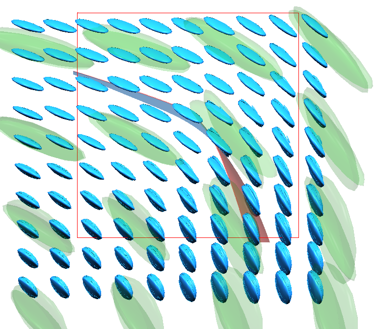
The above scenes depict the result when the Trend Type is set to Non-decaying. In these illustrations, a mesh has been selected and added to Trend Inputs and a trend Strength specified. Because the strength of the trend does not decay, all the ellipsoid disks are the same size but may point in different directions.
Creating a Structural Trend
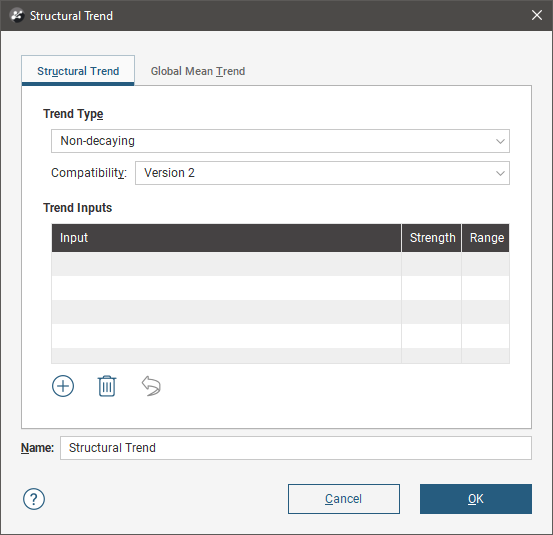
To create a new structural trend, right-click on the Structural Trends folder (in the Structural Modelling folder) and select New Structural Trend. The Structural Trend window will appear:
Structural trends can be created from surfaces and from structural data. Click Add to select from the suitable inputs available in the project. The list of inputs will be displayed:
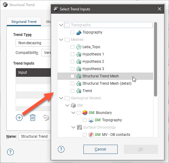
Tick the box for each input required, then click OK. The selected inputs will be added to the Structural Trend window:
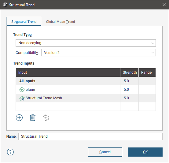
The Non-decaying option can be used when it can be assumed that the strength of the trend does not decay as you get further away from the mesh. This is useful when the geology has a fairly constant trend across the model, but with some directional shift. The Strength parameter describes how many times stronger the trend is in the maximum and intermediate plane than in the minimum direction. Note that when using a structural trend, the maximum and intermediate directions use the same strength value, so the depicted ellipsoids will always be oblate spheroids and cannot be prolate.
Where a trend is isolated to a region near a structure and the influence away from the structure decreases, an effect Range can be specified in conjunction with the Trend Type option Strongest along inputs. Where the trend approaches an isotopic trend, no ellipsoid is visualised.
Away from the structural trend, you can specify the overall global trend that the model should tend towards. The Global Mean Trend tab lets you set this as for a global trend, with Maximum, Intermed and Minimum ellipsoid ranges, and Dip, Dip Azimuth and Pitch directions. To set this, click on the Global Mean Trend tab.
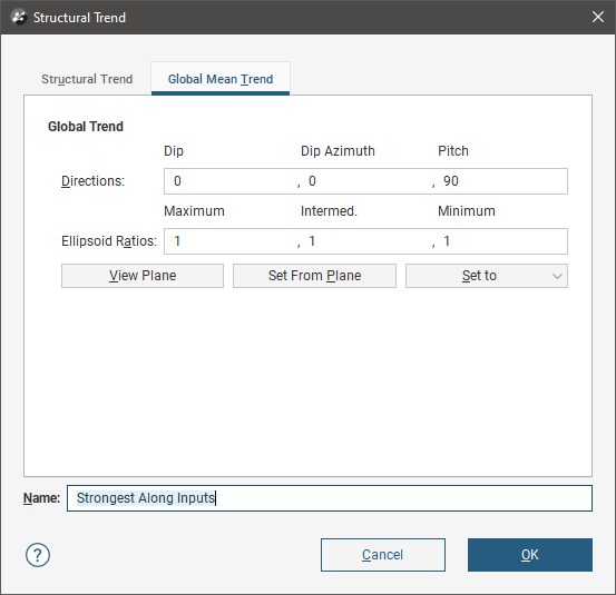
You can enter the trend manually or add the moving plane to the scene and set the trend using the moving plane, as described in Global Trends.
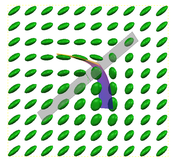
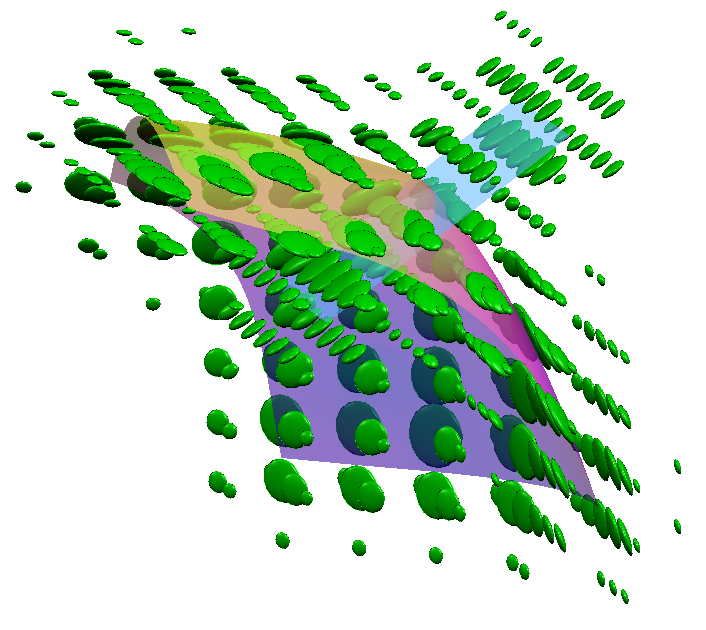
For instance, here a Strongest along inputs trend has been added to a global mean trend that goes in a very different direction.
Complex trend interactions can be modelled using structural trends by describing the trend components for each structure. Select Blending as the Trend Type, then add each input mesh to the Trend Inputs list, specifying an appropriate Strength and Range for each. The Blending option requires multiple meshes and blends them according to their individual strength settings. A trend with higher strength makes a stronger impact on the blending. The blended trend is a decaying type, and its strength weakens further away from the mesh. Leapfrog Geo will blend the trends at the places they interact. Because of the strength blending, some of these ellipsoids may end up prolate, but each of the component trend strengths can still only be configured using the same strength value for the maximum and intermediate directions. The Global Mean Trend tab can also be used to add an overall trend magnitude and orientation to the model.
Compatibility
Structural Trends includes an option to select the Compatibility as Version 1 or Version 2. Version 2 is the default and preferred option for all new models, as Version 1 is deprecated and retained for compatibility with existing, older models. Version 2 employs an improved strategy to ensure small changes such as the addition of a few new data points does not trigger a significant recalculation of the whole model. Both strategies use clusters of data with similar locations and trend orientations. These clusters are interpolated separately using the average trends across each cluster and then the interpolants are combined, smoothed with a weighed average. Version 1 recalculated the clusters whenever new data was added, potentially causing significant model changes from a small data change. Version 2 retains the clusters and only the clusters immediately surrounding the new data are updated, limiting the effect of the change.
The Compatibility setting determines the algorithm used to create the structural trend. Structural trends created in earlier versions of Leapfrog Geo (before 2.2) used the Version 1 algorithm. When these structural trends are upgraded, you can change them so they use Version 2, which may be desirable if adding more data to the trend results in significant changes in areas that are not close to new data.
Variable Orientation
For Kriging and other estimations, structural trends do not provide the needed control over the anisotropy ratios, among other considerations. For this purpose, Variable Orientation can be used.
This feature is only available when you have the Leapfrog Edge extension.
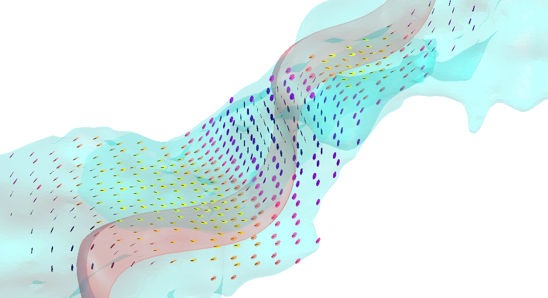
Variable orientation provides a similar control over the changing direction of anisotropy for the purposes of improving local value estimates, orienting the search space and variogram according to local characteristics. Variable orientation is visualised using lines or, as in this illustration, flat disks with a line indicating the orientation of the maximum axis direction for each search space local to each centroid. Here the disks have also been coloured reflecting the Dip direction.
For a full description of this feature, please see Variable Orientations.
Variography
This feature is only available when you have the Leapfrog Edge extension.
Variography is the analysis of spatial variability of grade within a region.
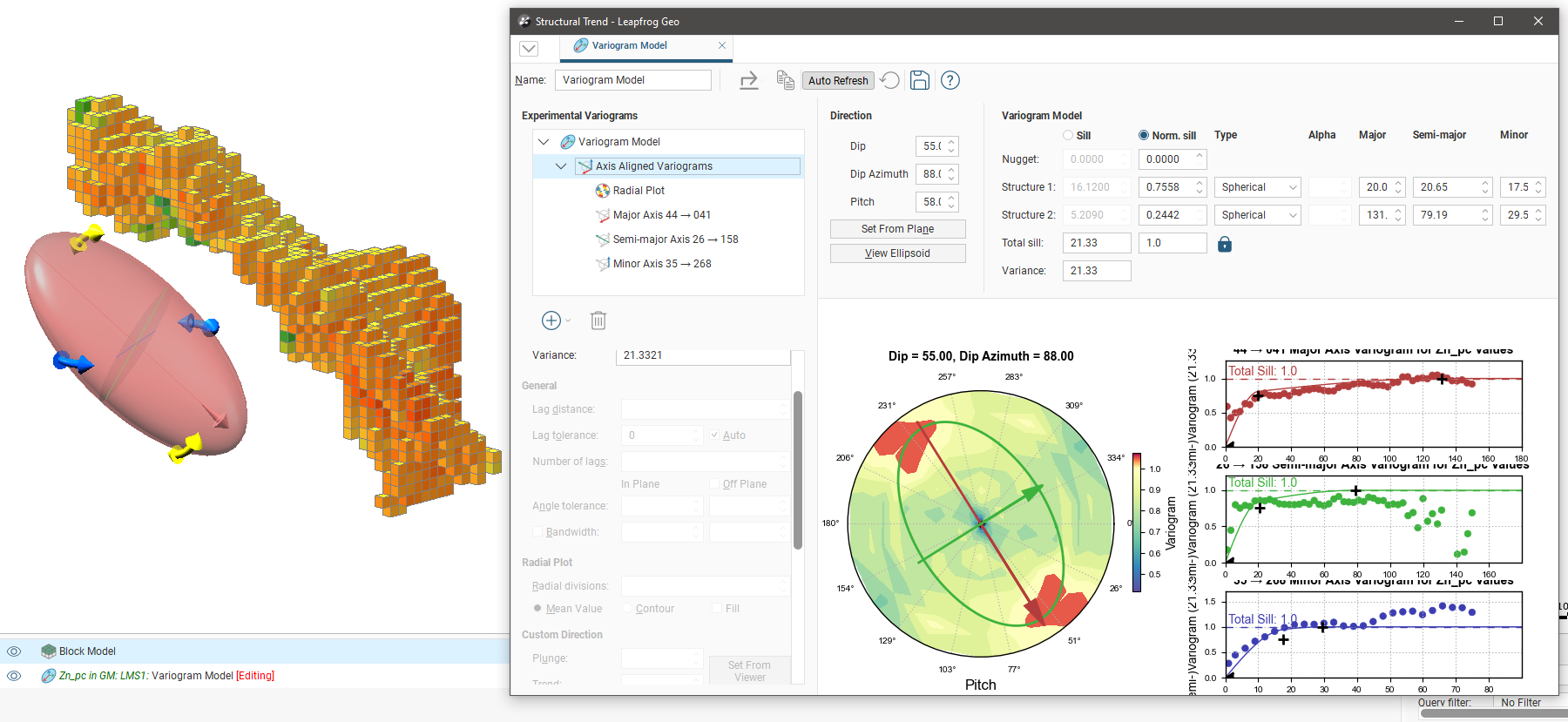
For more information on the variography capabilities in Leapfrog Edge, see Experimental Variography and Variogram Models.
Got a question? Visit the Seequent forums or Seequent support