Experimental Variography and Variogram Models
The features described in this topic are only available if you have the Leapfrog Edge extension.
Variography is the analysis of spatial variability of grade within a region. Some deposit types, e.g. gold, have high spatial variability between samples, whereas others, e.g. iron, have relatively low spatial variability between samples. Understanding how sample grades relate to each other in space is a vital step in informing grades in a block model. A variogram is used to quantify this spatial variability between samples.
In estimation, the variogram is used for:
- Selecting appropriate sample weighting in Kriging and RBF estimators to produce the best possible estimate at a given location
- Calculating the estimators’ associated quality and diagnostic statistics
In Leapfrog Geo domained estimations, variograms are created and modified using the Spatial Models folder. To create a new variogram model, right-click on the Spatial Models folder and select New Variogram Model.
A new variogram model is not auto-fitted and should not be assumed to be the initial hypothesis for the workflow. While some reasonable defaults have been selected for the variogram model, the geologist’s personal hypothesis should be the starting point for the estimation workflow.
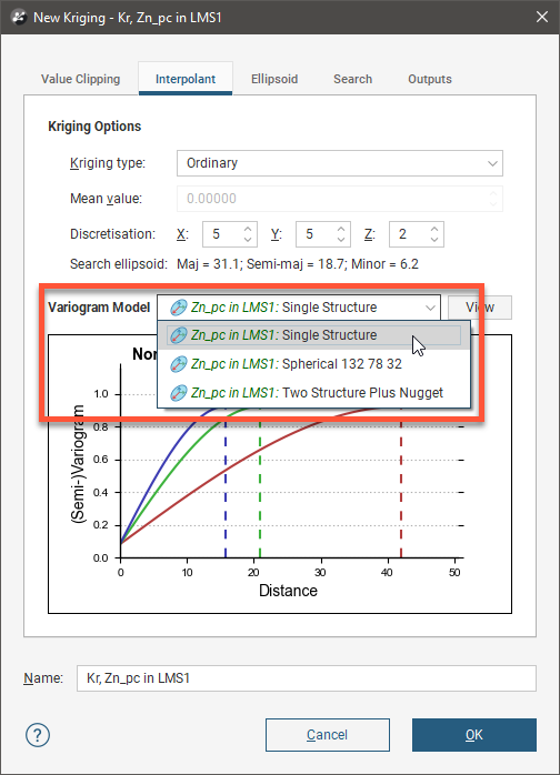
You can define as many variograms as you wish; when you define an estimator that uses a variogram model, you can select from those available in the contaminant estimation’s Spatial Models folder:
Working with variograms is an iterative process. The rest of this topic provides an overview of the Variogram Model window and describes how to use the different tools available for working with variograms. This topic is divided into:
See The Ellipsoid Widget for information that is useful in working in the Variogram Model window.
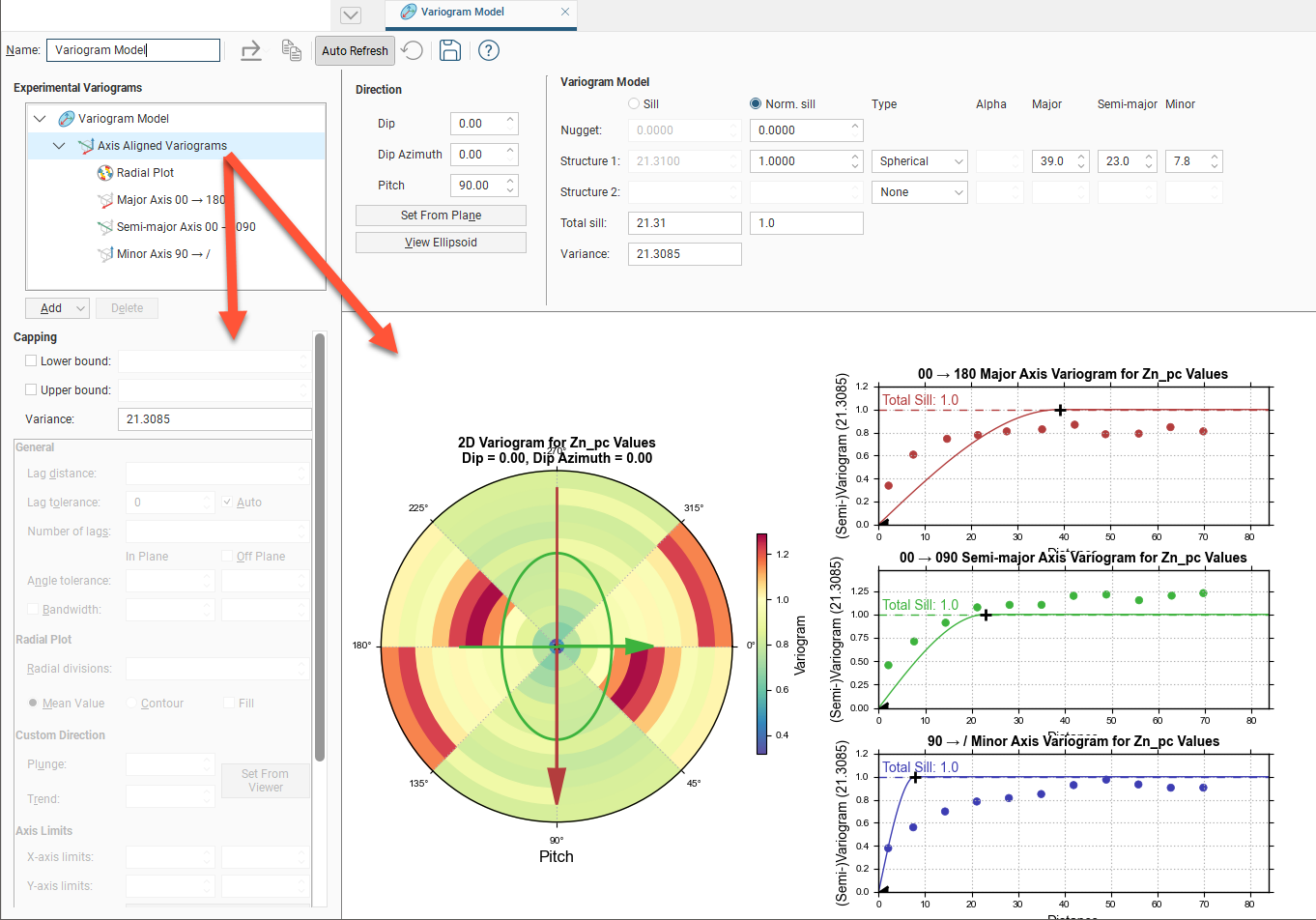
The Variogram Model Window
The Variogram Model window is divided into three parts:


|
Variogram model controls for adjusting the variogram model type, trend and orientation. See Variogram Model Controls below. |

|
Graphs plotting the selected variogram |

|
Experimental controls for verifying the theoretical variogram model. See Experimental Controls below. |
When you edit a variogram model in the Variogram Model window, an ellipsoid widget is automatically added to the scene. The ellipsoid widget helps you to visualise the variogram in 3D, which is useful in setting variogram rotation and ranges and in defining search neighbourhoods.
If the Variogram Model window is docked as a tab, you can tear the window off. As a separate window, you can move and resize the window so you can see the ellipsoid change in the 3D scene while you make adjustments to the model settings. The detached window can be docked again by dragging the tab back alongside the other tabs, as described in Organising Your Workspace.
There are two ways to save the graph for use in another application:
- Click the Export button (
 ) and select Export graph image from the options to export the graph as a PDF, PNG or SVG file.
 - Click the Copy graph button (
 ) to copy the graph to the clipboard. You can then paste it into another application.
Additionally, you can save variogram parameter data by selecting a theoretical variogram from the list, clicking the Export button (![]() ) and selecting Export data from the options. Note that Export data is not available for the experimental variogram or the Radial Plot.
) and selecting Export data from the options. Note that Export data is not available for the experimental variogram or the Radial Plot.

There are two buttons for refreshing the graphs when changes are made:
- When Auto Refresh is enabled, recalculations will be carried out each time you change a variogram value. This can produce a brief lag.
- When auto refresh is disabled, you can click the Refresh button (
 ) whenever you want the graphs to be updated. This is the best option to use when working with a large dataset.
If auto refresh is disabled and values have been changed without the graphs being updated, the chart will turn grey and a reminder will be displayed over it:

Variogram Model Controls
The Variogram Model controls adjust the variogram model type, trend and orientation; the graph will update to reflect changes you make to model parameters. The ellipsoid in the scene will also reflect the changes you make to the Variogram Model.
Multi-structured variogram models are supported, with provision for nugget plus two additional structures.
The Nugget represents a local anomaly in values, one that is substantially different from what would be predicted at that point based on the surrounding data. Increasing the value of Nugget effectively places more emphasis on the average values of surrounding samples and less on the actual data point and can be used to reduce noise caused by inaccurately measured samples.
Each additional structure has settings for the component Sill and the normalised sill, labelled Norm. sill, model Type, Alpha (if the model type is spheroidal), and the Major, Semi-Major and Minor ellipsoid ranges.
The Sill defines the upper limit of the model, the distance where there ceases to be any correlation between values. The Sill can be set for the Nugget, Structure 1 and Structure 2.
Piecewise models rise to the Sill at the Range and stay there for increasing distances beyond the Range. Distances beyond the Range in the domain are uncorrelated.
Asymptotic models approach the sill asymptotically near the range and continue to approach it for increasing distances beyond the range. For asymptotic models, the Range parameter used in the model has no equivalent physical meaning, as it does for piecewise models. Common practice is to instead use a scaling of the Range parameter so that the value entered in this screen somewhat mimics the sill/range behaviour of a piecewise model. Typically, this scaling parameter is chosen so that the ‘practical range’ or ‘effective range’ entered corresponds to a point on the asymptotic function that is a defined percentage of the total sill. There is no universally accepted way of defining what this scaling parameter should be. The practical range used in Leapfrog Geo is noted below for each variogram model Type.
A linear model has no sill in the traditional sense, but, along with the ellipsoid ranges, the sill sets the slope of the model. The two parameters Sill and Range are used instead of a single gradient parameter to permit switching between interpolant functions without also manipulating these settings.
The Norm. sill represents the same information as the Sill, but proportionally scaled to a range between 0 and 1, where 1 represents the data Variance. As you select the radio buttons for Sill and Norm. sill, the Y-axis scale on the displayed chart will change to correspond to your selection.
The Total sill is the sum of the component sills for both the data sills and the normalised sills.
The Lock sill icon indicates if the sill is unlocked (![]() ) or locked (
) or locked (![]() ). Click the icon to change the lock state. If unlocked, changing a sill value will adjust the Total sill by the same amount. If locked, adjusting any sill value will not change the Total sill at all, but other sill values will change to keep the Total sill fixed.
). Click the icon to change the lock state. If unlocked, changing a sill value will adjust the Total sill by the same amount. If locked, adjusting any sill value will not change the Total sill at all, but other sill values will change to keep the Total sill fixed.
The Variance is calculated automatically from the data and shows the magnitude of the variance for the dataset.
Model Options
Leapfrog Geo provides a variety of ‘authorised’ variogram model types to ensure the spatial character of continuity can be modelled. ‘Authorised’ variogram models are guaranteed to have the mathematical property of ‘positive definiteness’ for the associated covariance function, meaning the model is guaranteed to produce a valid result when used in Kriging. The model Type provides the options Linear, Spherical, Spheroidal, Gaussian, Exponential, Cubic and Generalised Cauchy.
Variogram models can be bounded or unbounded. Linear is the only unbounded type provided by Leapfrog Geo, where the value of the variogram increases as a linear function of distance. Linear models cannot be combined with the bounded models.
All other model types provided in Leapfrog Geo are bounded models that rise to a sill. These can be separated into two further types:
- Piecewise models that rise to a sill at a range, then are constant beyond that range
- Asymptotic models that approach but never reach a sill
Spherical and Cubic models are piecewise; Spheroidal, Gaussian, Exponential and Generalised Cauchy are asymptotic.
The functions vary in how quickly they rise toward the sill both initially and at (and beyond) the range.
Which function you select will depend on the variable you are modelling, as well as the performance required. For instance, Generalised Cauchy is provided as it is faster than the Gaussian function when applied to an RBF estimator, but provides reasonably similar results.

Variogram model types Cubic, Gaussian and Generalised Cauchy are included specifically for modelling variables with high continuity and local correlation such as dispersed groundwater contaminants. Screening effects and negative Kriging weights can be more pronounced when using these models with continuous behaviour, so use the block model interrogation tool to check the Kriging plan is optimal and the Kriging weights are appropriate.
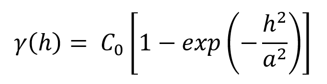
Each of the variogram model Types are described below. For each, a formula is presented for the model. They all use the following terms:
- γ(h) is the value of the variogram at distance h
- C0 is the sill
- h is the distance on the x axis
- a is the range parameter
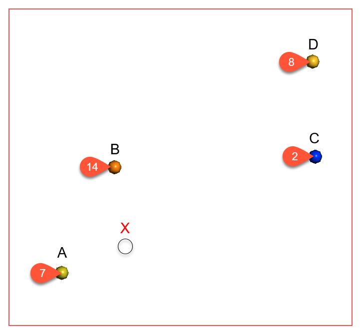
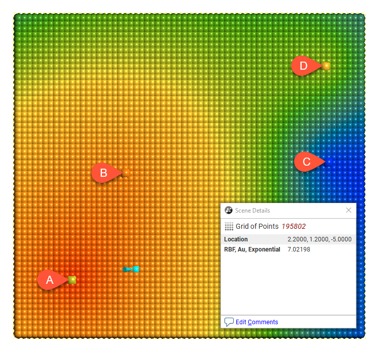
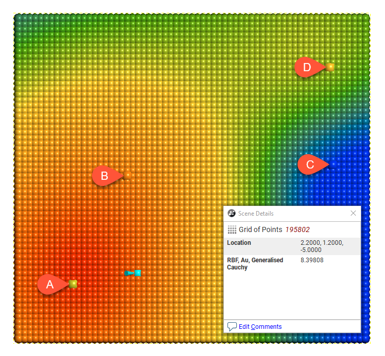
For each model type, the effect of the interpolation function is depicted by evaluation onto a grid of points, using as input just four samples, A = 7, B = 14, C = 2 and D = 8. A thin slice is taken through the grid of points to provide a sort of 2D visualisation of the operation of the function. One of the points has been selected in each view to display the value being estimated for a specific location.
Type = Linear

Linear is a general-purpose multi-scale option suited to sparsely and/or irregularly sampled data. It is typically used for modelling of categorical variables.

Type = Spherical
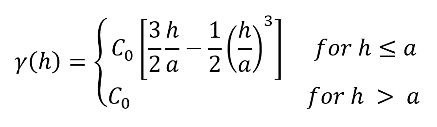
Spherical is suitable for modelling most variables where there is a finite range beyond which the influence of the data should fall to zero. Because the spherical model is piecewise, beyond the range the variogram value is the constant sill.

Type = Cubic

Cubic, like Spherical, is a piecewise model that has a finite range beyond which the influence of the data should fall to zero, and the variogram value is the constant sill. It has been included specifically for modelling variables with high continuity and local correlation such as dispersed groundwater contaminants. Screening effects and negative Kriging weights can be more pronounced when using the cubic model type with continuous behaviour, so use the block model interrogation tool to check the Kriging plan is optimal and the Kriging weights are appropriate.

Type = Exponential
The Exponential variogram model type is used in modelling precious metals such as gold. It has a steeper slope toward the origin than other model types.
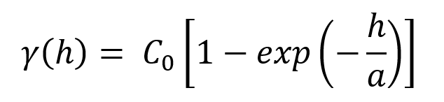
The Exponential model is asymptotic and approaches but never quite reaches the Sill.
An exponential model with a range parameter of a reaches a value of ~95% of the sill at a distance of 3 x a. The Range value is scaled by a factor of 1/3 in the formulation. This has the effect of ensuring that the exponential variogram reaches ~95% of the sill at the ‘practical range’. Beyond the practical range, a point has a small but non-zero correlation.
Type = Gaussian
The Gaussian model is asymptotic and approaches but never quite reaches the Sill.
Gaussian has been included specifically for modelling variables with high continuity and local correlation such as dispersed groundwater contaminants. Screening effects and negative Kriging weights can be more pronounced when using these models with continuous behaviour, so use the block model interrogation tool to check the Kriging plan is optimal and the Kriging weights are appropriate.
A Gaussian model with a range parameter of a reaches a value of ~95% of the sill at a distance of √3 x a. The Range value is scaled by a factor of 1/√3 in the formulation. This has the effect of ensuring that the Gaussian variogram reaches ~95% of the sill at the ‘practical range’. Beyond the practical range, a point has a small but non-zero correlation.

Type = Generalised Cauchy
The Generalised Cauchy model is asymptotic and approaches but never quite reaches the Sill.
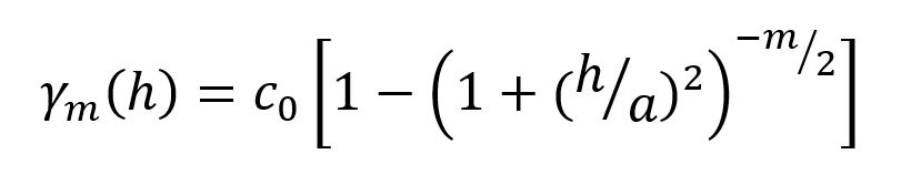
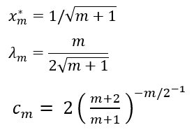
The Generalised Cauchy covariance can be expressed as:
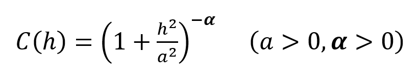
By considering only particular values for the exponent α this expression can be simplified to derive a standardised Generalised Cauchy covariance function of order m, where m = 2α
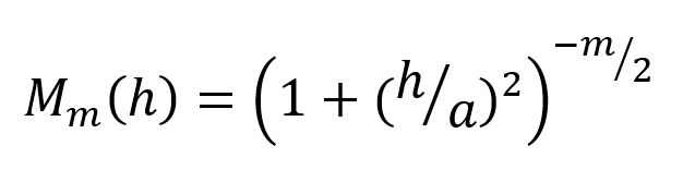
This can in turn be expressed as a variogram function for the Generalised Cauchy variogram of order m:
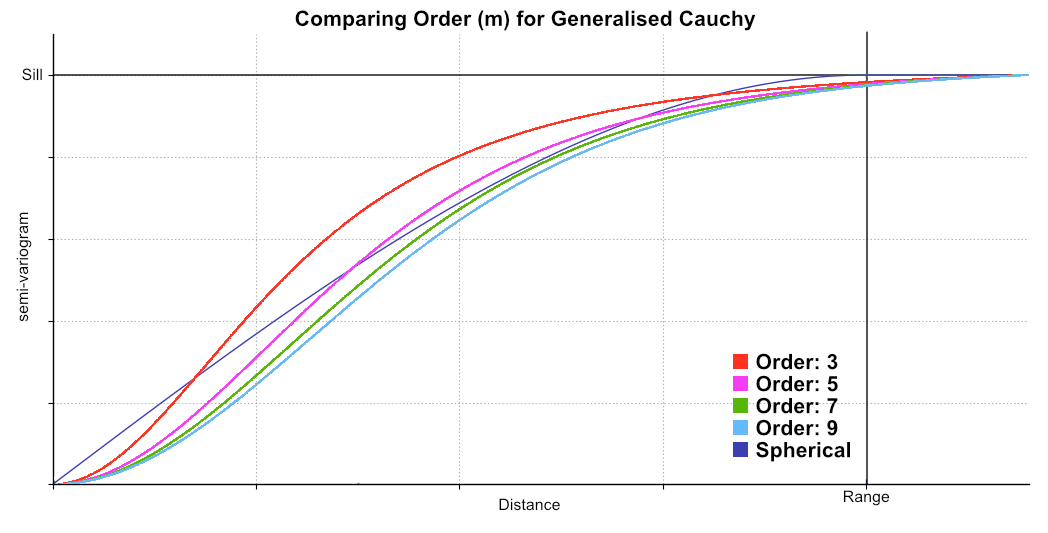
Select the order m by selecting from the Alpha options of 3, 5, 7 or 9, which are the only values allowed in Leapfrog Geo. For a given range parameter a, the variograms of order m reach the same proportion of total sill at quite difference distances. In order to equate the shape of the variogram to the entered Range parameter, scaling parameters are applied.
For a Generalised Cauchy variogram of order 9, the value of γ at the specified range parameter is 95.58% of the total sill. Because the convention is arbitrary, Leapfrog Geo considers that a variogram of order 9 does not require a re-scaling of the range parameter. Leapfrog Geo then uses this sill proportion of 95.58% to calculate scaling factors for variograms of order 3, 5 and 7. In practice, a lookup table is used with ideal values rounded to 10 decimal places:
| Order (m) | Range scaling factor |
| 3 | 0.3779644730 |
| 5 | 0.6347188807 |
| 7 | 0.8339047224 |
| 9 | 1.0000000000 |
This has the effect of ensuring that the Generalised Cauchy variogram reaches 95.58% of the sill at the ‘practical range’. Beyond the practical range, a point has a small but non-zero correlation. For further details on the derivation see The Spheroidal Family of Variograms Explained on the Seequent blog.
This chart shows the relative differences for different values of Alpha, which is the order (m) of the function, in comparison to a spherical curve:
Type = Spheroidal
The Spheroidal model is asymptotic and approaches but never quite reaches the Sill. However, the first part of the function is linear.
Spheroidal is suitable for modelling most variables where there is a finite range beyond which the influence of the data should fall to zero. The spheroidal variogram was developed by Seequent primarily for use in RBF interpolants. Seequent wanted an effectively compact spatial function that has linear behaviour near the origin and an asymptotic approach to the sill. This was developed by taking a commonly used family of radial functions and linearizing them near the origin. This results in a variogram that combines the Linear model with the Generalised Cauchy variogram model. The transition point between these two is the inflection point on the Generalised Cauchy model.
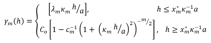
where
Select the order m by selecting from the Alpha options of 3, 5, 7 or 9, which are the only values allowed in Leapfrog Geo. For a given range parameter a, the variograms of order m reach the same proportion of total sill at quite difference distances. In order to equate the shape of the variogram to the entered Range parameter, scaling parameters are applied.
For a Spheroidal variogram of order 9, the value of γ at the specified range parameter is 96% of the total sill with no nugget. Because the convention is arbitrary, Leapfrog Geo considers that a variogram of order 9 does not require a re-scaling of the range parameter. Leapfrog Geo then uses this sill proportion of 96% to calculate scaling factors for variograms of order 3, 5 and 7. In practice, a lookup table is used with ideal values rounded to 10 decimal places:
| Order (m) | Range scaling factor |
| 3 | 0.3731574337 |
| 5 | 0.6319995630 |
| 7 | 0.8327312240 |
| 9 | 1.0000000000 |
This has the effect of ensuring that the Spheroidal variogram reaches 96% of the sill at the ‘practical range’ with no nugget. Beyond the practical range, a point has a small but non-zero correlation. For further details on the derivation see The Spheroidal Family of Variograms Explained on the Seequent blog.
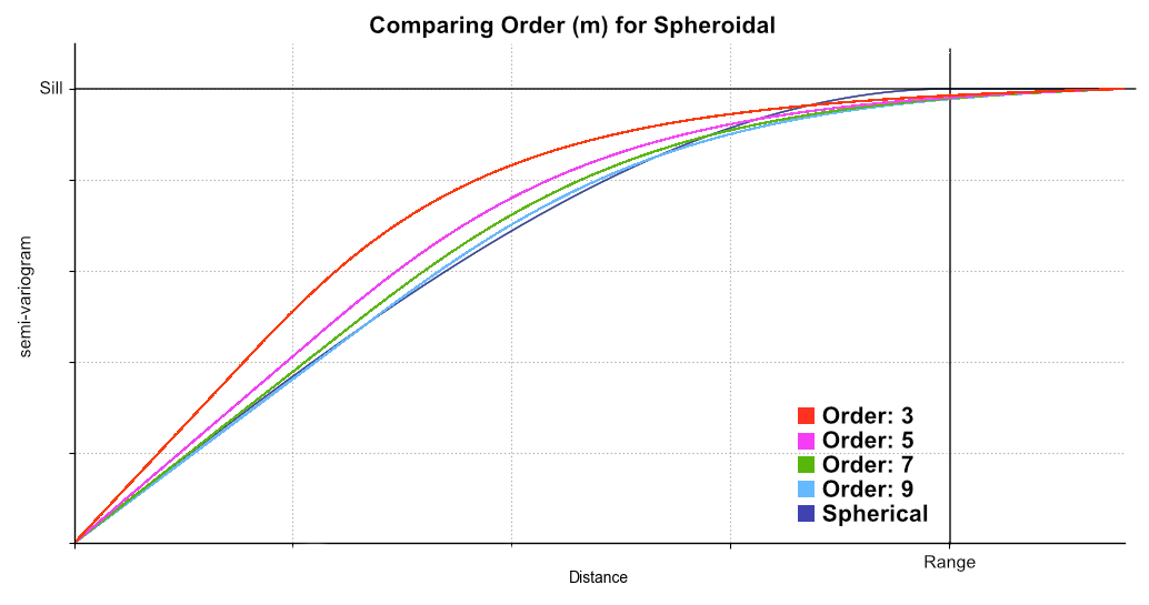
This chart shows the relative differences for different values of Alpha, which is the order (m) of the function, in comparison to a spherical curve:

The spherical model is not available for standard Leapfrog RBF interpolants created in the Numeric Models folder.
Alpha is only available when the model Type is Spheroidal or Generalised Cauchy. The Alpha constant determines how steeply the interpolant rises towards the Sill. A low Alpha value will produce a variogram that rises more steeply than a high Alpha value. A high Alpha value gives points at intermediate distances more weighting, compared to lower Alpha values. An Alpha of 9 provides the curve that is closest in shape to a spherical variogram. In ideal situations, it would probably be the first choice; however, high Alpha values require more computation and processing time, as more complex approximation calculations are required. A smaller value for Alpha will result in shorter times to evaluate the variogram.
RBF estimators will only work when the Structure 2 model Type is set to None.
When Structure 2 is defined, the model ranges cannot be adjusted by manipulation of drag handles on the ellipsoid. Because it would not be clear which structure was being manipulated, the drag handles to change the range settings do not appear.
Normalised Y Axis
A key use of copying a variogram is to apply it to another correlated contaminant. This would typically be accomplished, having determined the appropriate variogram using the values for one contaminant, by copying the domained estimation and changing the Numeric values field to a different contaminant. However, the absolute values for the nugget and sills for each structure would be completely inappropriate for the new contaminant; while we desire the shape to be the same, the values for different compounds will inevitably be different. To make this work correctly, the variogram is normalised or standardised, rescaling the range of Y-axis values to between 0 and 1, where 1 is equivalent to the data Variance. This makes the variogram information portable between domained estimations. This is performed automatically, requiring no intervention on your part.
You can freely switch between the Sill and Norm. sill options. The selection only changes the Y-axis scale on the displayed chart.
You do not need to select the Normalised option before copying the domained estimation and using it as the basis for a different mineral resource. The normalised scale will always be used when applying the variogram model to the new data set.
As you adjust the Nugget or the Structure 1 or Structure 2 sill values, the Total sill will change both for the absolute Sill values and the Norm. sill values. The Norm. sill total may end up being something other than 1.0. This is expected, as the value reference for the normalised scale uses the data Variance for 1.0, not the total sill.
Note that the data Variance is recorded in the Y axis label so the chart scale is always meaningful, including when the chart is exported.
Direction
The trend Direction fields set the orientation of the variogram ellipsoid. Adjust the ellipsoid axes orientation using the Dip, Dip Azimuth and Pitch fields.
The Set From Plane button sets the trend orientation of the model ellipsoid based upon the current settings of the moving plane.
The View Ellipsoid button adds a 3D ellipsoid widget visualisation to the scene, in case it has been deleted from the scene since the variogram model window was opened for editing.
Experimental Controls
A variogram model can be verified through the use of the experimental variography tools that use sample data. Use these to find the directions of maximum, intermediate and minimum continuity.
The variogram displayed in the chart is selected from the variograms listed in the panel in the top left corner of the window.
The top entry in the variograms list is the theoretical variogram model rather than an experimental variogram:
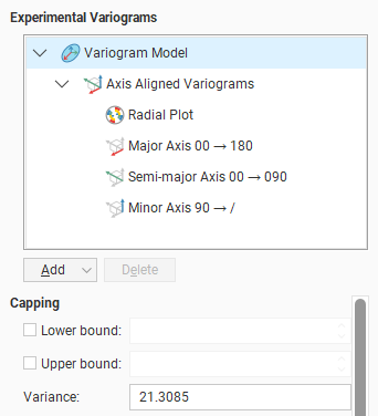
All other variograms in the list and the other controls on the left-hand side of the screen relate to Experimental Variograms.
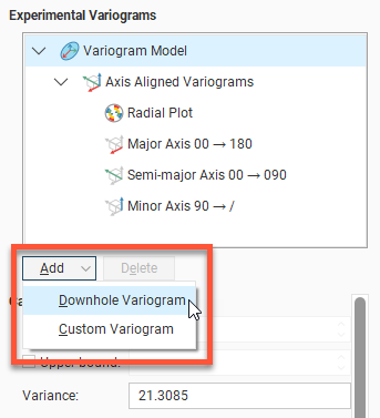
By default, there is a set of Axis Aligned Variograms. Use the Add button to add additional experimental variograms. You can add one Downhole Variogram and any number of Custom Variograms.
Click on one of these experimental variograms to select it and display its parameters. The displayed graph will change to match this selection. For example, here the graph and settings for the combined Axis Aligned Variograms are displayed:
Selecting the Semi-major Axis variogram changes the chart and settings displayed:
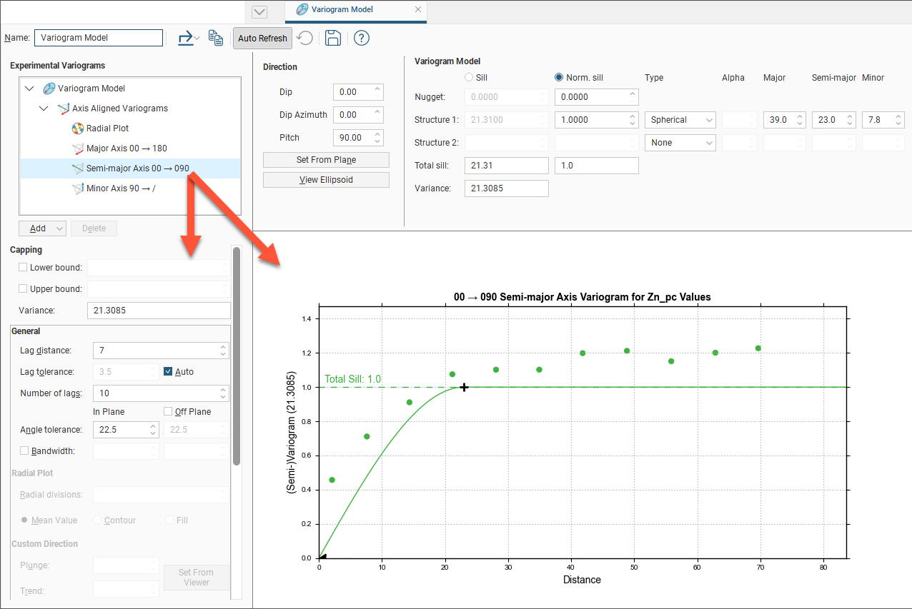
Adjust the model variogram parameters to see the effect different parameters have when applied to the actual data.
Experimental Variogram Parameters
The experimental variogram controls along the left side of the window define the search space, define the orientation for custom variograms and change how the variograms are displayed. Some parameters are only available for some variogram types; these are discussed in later sections on each variogram type.
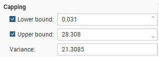
Capping
Data Capping fields limit the values of the Lower bound and Upper bound for the data as specified. This is not a filter that discards these points, but values below or above the caps are treated as if the value was the lower or upper bound.
These Capping controls only affect the data values considered for the purposes of experimental variography, and they do not cap the values of the data points used in estimation. If you wish to also cap values used in estimation, set the Lower bound and Upper bound limits in the Value Clipping tab in the applicable estimator. To eliminate an anomalous data point or discard certain data values, you should modify the domain definition options using a Query Filter.
Defining the Search Space
The search space for experimental variography is not shown in the scene. It is not an ellipsoid, and should not be confused with either the variogram model ellipsoid or the estimator's search ellipsoid.
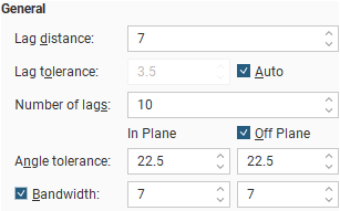
The first set of parameters controls the search space.
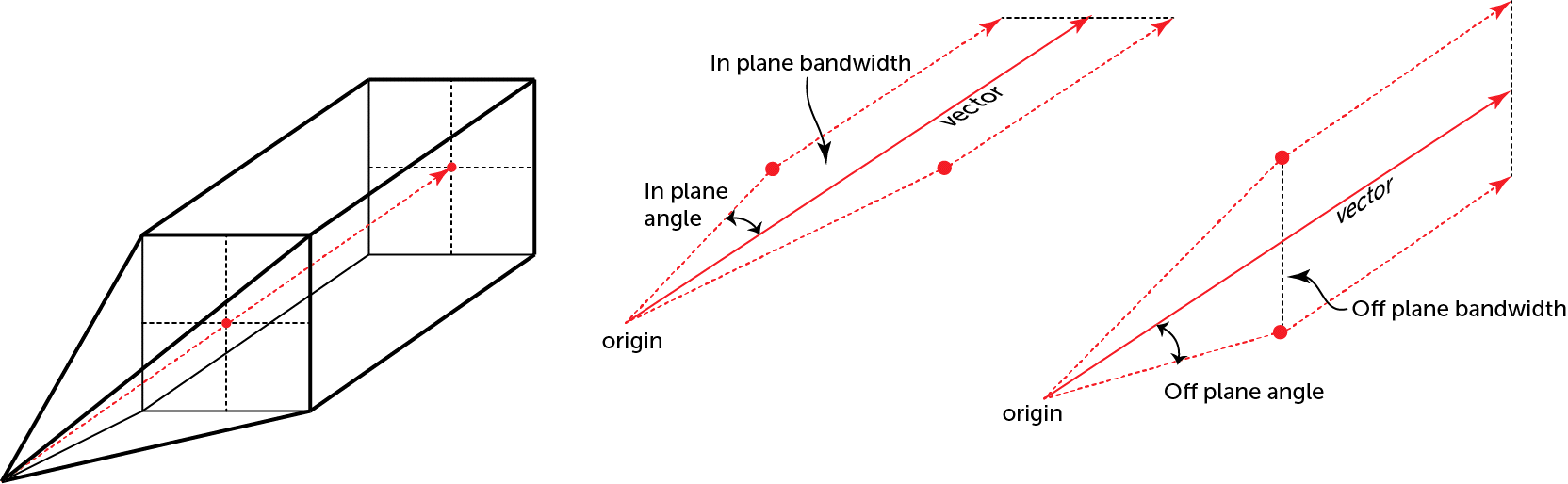
- Lag distance controls the size of the lag bins. The first bin will be one quarter of the size of the Lag distance. Experimental variograms generally measure lags as distances along a direction vector, though downhole variograms measure lags as distances along the drillholes.
- Lag tolerance allows for the reality that data pairs are rarely the same distance apart. The data is scanned and pairs are assembled after applying a Lag tolerance to the Lag distance. If the Lag tolerance Auto box is ticked, Leapfrog Geo defaults to using a Lag tolerance of half the Lag distance. Controlling the Lag tolerance explicitly allows you to test the sensitivity of the variogram. Typically, a larger value will be used for sparse datasets and a smaller value for dense datasets.
Some software treats a Lag tolerance of 0 as a special value that does not mean ‘no lag tolerance’ but instead is interpreted as meaning half the Lag distance. In Leapfrog Geo, it is possible to set Lag tolerance to 0, but this means literally what the number implies: there is no Lag tolerance and the only data pairs that are displayed are those that occur exactly at the Lag distance spacing.
- Number of lags constrains the number of lag bins in the search space.
- The In Plane and Off Plane Angle tolerance and Bandwidth settings define the search shape, and the effects of these settings are discussed in more detail below.
The search shape usually approximates a right rectangular pyramid on a rectangular parallelepiped. The pyramid and parallelepiped will be square if the In Plane Angle tolerance and Bandwidth are used without defining Off Plane values. Using the Off Plane Angle tolerance and Bandwidth fields will make the shape rectangular. The plane being referred to is the major-intermediate axis plane of the variogram ellipsoid, the same plane used for the radial plot. The Angle tolerance is the angle either side of a direction vector from the data point origin. Once the sides of the pyramid defined by the angle tolerances extend out to the limits specified by the Bandwidth, the search neighbourhood is constrained to the bandwidth dimensions.
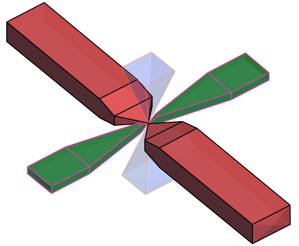
The search shape becomes a more complex “carpenter’s pencil” shape when a wide In Plane angle and a narrow Bandwidth are defined along with a narrow Off Plane angle and a wide Bandwidth, or vice versa. This rendering should assist in visualising the shape; the major axis is shown in red, the semi-major axis is shown in green, and the orthogonal minor axis in a transparent blue:
Note that although not shown here, the outer ends of the search shapes are not flat, but rounded, being defined by the surface of a sphere with a radius of the maximum distance defined by the number of lags and their size.
Off Plane Angle tolerance and Bandwidth settings cannot be set for the minor axis variogram. Because the angle tolerance and bandwidth are described relative to the major-intermediate plane and because the minor axis is orthogonal to this plane, only one angle can be described. This results in a square pyramid search shape.

The In Plane Bandwidth also cannot be set for the Minor Axis.
Note that although not shown here, the outer ends of the pyramids are rounded, defined by the surface of a sphere with a radius of the maximum distance defined by the number of lags and their size.
Radial Plot Parameters
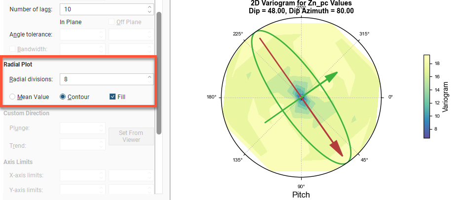
Radial Plot has parameters specifically for the radial plots in Axis Aligned Variograms.
Increasing the Radial divisions slices the space into a larger number of sectors, with each block in the radial plot covering a smaller arc of the compass. As a result, each block has a smaller volume; this also means that the amount of data in each block is reduced. Because the bandwidth angle above and below the major-intermediate plane matches the angle used to slice the plot into its sectors, increasing the Radial divisions also reduces the number of data points used above and below the plane. Using a smaller number of Radial divisions will be faster. If you increase the number of divisions, you may want to turn off Auto Refresh Graphs first and click Refresh graphs afterwards. Experiment with the number of divisions and choose the lowest number of Radial divisions that helps you gain the best understanding of continuity; this will maximise the data that falls in each division.
Mean Value will display radial plot bins coloured to indicate the mean value for each bin. Contour will display a plot showing lines of equal value. Fill shades the chart between the contour lines.
Orienting Custom Variograms
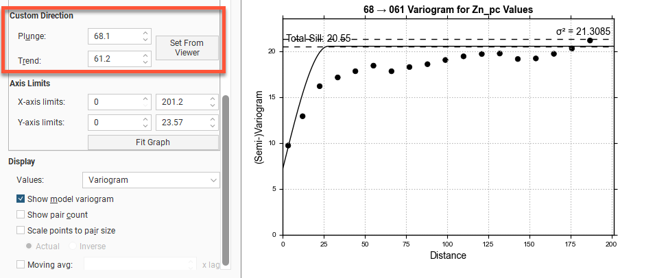
The Custom direction fields are for Custom Variograms that use the Plunge to Trend settings to orient the variogram trend. They can easily be set by orienting the scene view and then clicking the Set From Viewer button, which sets the plunge and trend to that of the scene view.
Changing Axis Limits
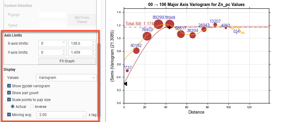
The Axis Limits settings control the chart scaling.
X axis limits and Y axis limits control the ranges for the X-axis and Y-axis and can effectively be used to zoom the chart. You can directly control these by manipulating the axes with your mouse. Click and drag an axis to increase or decrease the maximum limit of the axis. Right-click and drag an axis to reposition the axis so the minimum value on the axis is not zero. Double-click the axis to reset the axis minimum and maximum range to the default values. Fit Graph will auto-fit the graph to the available data.
Changing Variogram Display
The Display settings change how the variogram is displayed:
- Values offers a variety of options to plot on the chart: Variogram, Correlogram, Covariance, Relative Variogram and Pair-wise Variogram.
- Show model variogram plots the variogram on the chart.
- Show pair count annotates the chart with the count of data point pairs.
- Tick the Scale points to pair size checkbox and the chart will display the plotted points with dots that scale to the size of the pair count. Choose Actual so the dots represent the pair size proportionally and Inverse to see larger dots for lower pair counts.
- Tick Moving avg for a rolling mean variogram value, drawn on the variogram plots in orange. Next to it, select a value for the window size relative to the Lag distance.The window size will be the given number times the lag distance. This window, centred on x, will be used to plot y, the average of all the variogram values falling inside the window. The lag multiplier field has a useful tooltip reminder; hover your mouse pointer over the field to see the tooltip.
The Downhole Variogram
The Downhole Variogram can be used to better define the nugget. It looks only looks at pairs of samples on the same drillhole and uses the differences in depths to calculate the lag value.
As it isn’t associated with a specific direction, the Angle tolerance parameter is not available for the Downhole Variogram.
The Downhole Variogram chart does not plot the model variogram line; instead it shows a dotted horizontal line indicating the Total Sill and, if Sill is chosen instead of Normalised Sill, the variance.
A model is not fitted to the Downhole Variogram data because not all drillholes are oriented in the same direction. An alternative that provides a fixed direction is to use a Custom Variogram. Adjust the scene to look down a specific drillhole in the relevant direction, then choose Set From Viewer to set the Plunge to Trend values.
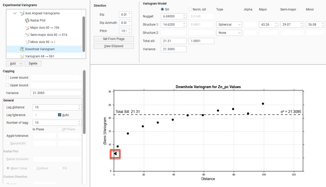
A triangular dragger handle next to the chart’s Y-axis can be used to adjust the Nugget value in the Model Controls part of the window. As the downhole values are nearly continuous, an accurate estimate can be made for the nugget effect for this direction.
Axis Aligned Variograms
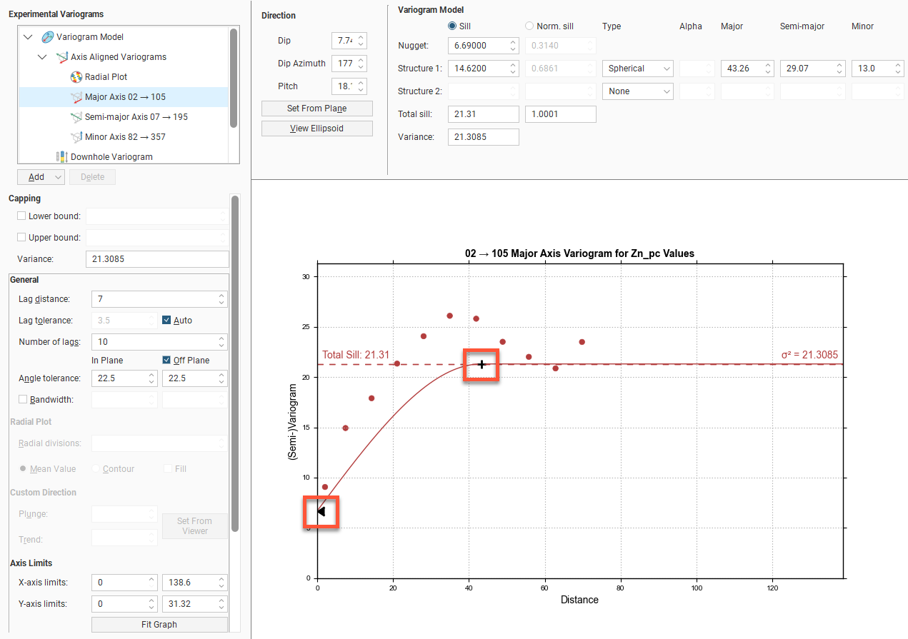
The Axis Aligned Variograms are useful for determining the direction of maximum, intermediate and minimum continuity. When you select the Axis Aligned Variograms option, all four variograms are displayed in the chart:

The radial plot and each of the axes variograms can be viewed in greater detail by clicking on them in the variogram tree:
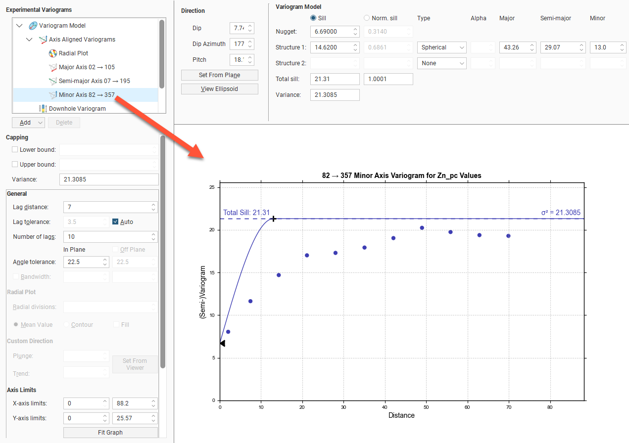
In the axes variogram plots, you can click-and-drag the plus-shaped dragger handle to adjust the range and the sill. A triangular dragger handle adjusts the nugget. A solid line shows the model variogram, and dotted horizontal lines show the Total Sill and, if Sill is chosen instead of Norm. sill, the variance.
Drag handles do not appear on the plots for all display Values options. Handles are not provided for Pairwise Relative because fitting models to pairwise relative variograms is discouraged in the industry. The reason this is discouraged is because the calculation provides a distinctly non-linear re-scaling of the variogram and suppresses the effect of outliers, producing a variogram that is usually optimistic with respect to both nugget and range of continuity.
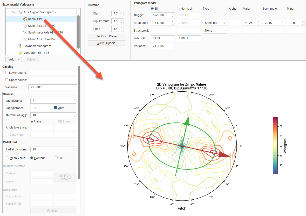
In the radial plot, you can click-and-drag the axes arrows to adjust the pitch setting, between the values 0 and 180 degrees. Each bin in the mean value radial plot shows the mean semi-variogram value for pairs of points binned by direction and distance. When the contour plot is selected, lines follow the points of equal value.
The experimental variogram controls can be different for each axis direction.
Custom Variograms
Any number of custom variograms can be created. These are useful when validating a model, for checking the variogram directions other than the axis-aligned directions. The Plunge to Trend settings determine the direction of the experimental variogram, and these are set independently of the Dip, Dip Azimuth and Pitch settings used by the other experimental variograms. The Plunge to Trend settings can be quickly set by orienting the scene and then clicking the Set From Viewer button in the Variogram Model window. This copies the current scene azimuth and plunge settings into the fields for the custom variogram.
When selected, the custom variogram shows a semi-variogram plot, with the model variogram plotted:

There are no handles on this chart. Dotted horizontal lines indicate the Total Sill and, if Sill is chosen instead of Norm. sill, the variance.
Got a question? Visit the Seequent forums or Seequent support