Grid using TIN

Use the Grid and Image > Gridding > Tinning > Grid using TIN menu option (TINGRID GX) to create a TIN grid from a Z-valued Triangular Irregular Network (TIN).

Grid using TIN dialog options

Input TIN File	The name of the serialized TIN file. Script Parameter: TINGRID.FILE
Output grid	Name of the file to write the TIN information to. This is a binary file and cannot be read using a text editor program. The saved file can then be used as input to other GXs, such as TINMESH. Script Parameter: TINGRID.GRID
Interpolation method	Linear: triangles in the TIN are interpolated using a plane defined by the triangle vertices. Natural Neighbour: uses the Natural Neighbour algorithm described by Sambridge et al (1995)¹. Nearest Neighbour: uses the values of the nodes closest to the given locations. Script Parameter: TINGRID.METHOD: 0: Linear, 1: Natural Neighbour; 2: Nearest Neighbour (default 1)
Grid cell size	The size of the cells in the output grid. If this value is not specified, a default is chosen, based on the average density of points in the TIN. (The cell size is chosen to give a density about twice this value). Script Paramter: TINGRID.CELL

Application Notes

Gridding with Natural Neighbours

$image\tinning1.jpg$

Figure 1: The Voronoi diagram for a set of 16 nodes in a plane.

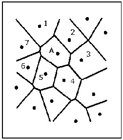
The natural neighbours of any node are those in the neighbouring Voronoi cells, or equally, those to which the node is connected by the sides of Delaunay triangles. For example in Figure 1, node A has natural neighbours numbered 1 to 7. The importance of natural neighbours is that they represent a set of ‘closest surrounding nodes’ whose number and positions are well defined and vary according to the local nodal distribution.

Natural neighbours can be thought of as a unique set of nodes that defines the ‘neighborhood’ of a point in the plane. If the distance between nodes is relatively large in some places, or small in others, the set of natural neighbours will reflect these features, but still represent the best set of nearby surrounding nodes. They are therefore ideal candidates for the basis of a local interpolation scheme; the equation [Sambridge & all, 1995]¹ is as follows:

$image\img00034.jpg$

Where:

f (x,y) is the interpolated function value.

f_i (i=1….,n) is the data value at the n natural-neighbour nodes to the point (x,y).

$image\img00035.jpg$ (i=1,…..,n) is the weight associated with each node.

The method in which the weights $image\img00036.jpg$ are determined controls the smoothness properties of the interpolation. However, since the summation (in the equation above) is only over the natural-neighbour nodes, then, regardless of how the $image\img00037.jpg$ are determined, the interpolation is guaranteed to be local. Furthermore, the size and shape of the region that can influence any point will adapt naturally to the local variation in node density. The natural neighbour grid has the desirable property that locations which fall exactly on a TIN node have exactly the value of that node, and the interpolation is smooth in the first derivative.

The TIN must be Z-valued; that is each X,Y location must have a corresponding Z-value. The TINDB GX automatically creates a Z-valued TIN.

Reference

The Natural Neighbour algorithm is described in the following paper:

[1] Malcolm Sambridge, Jean Braun, Herbert McQueen, "Geophysical parametrization and interpolation of irregular data using natural neighbours", Geophysical Journal International , vol. 122, no. 3 (December 1995), pp. 837-857.
DOI: https://doi.org/10.1111/j.1365-246X.1995.tb06841.x.