Coordinate System

The Coordinate System dialog is called through a wizard to allow you to set, inspect, or modify the parameters of the coordinate system (CS) specified in the previous dialog.

Coordinate channels or geolocated file name

Depending on where this dialog is called from, this non-editable field shows the existing or new abscissa & ordinate database channels or the current file name. The information that follows pertains to the CS of the channels or to the CS of the file.

Coordinate System

Well-known ID	This non-editable entry is populated with the standard EPSG name of the current CS, should there be one associated with this CS. This field will remain blank otherwise. When the coordinate system is modified, the reset button will appear to the right of this field. Press the button to reset the CS to its previous settings.
[Details...]	Click on this link to display a comprehensive list of the CS parameters.
Type	This non-editable field shows if the associated coordinates are in a Geographic or Projected coordinate system. If the coordinate system is not set, this field will display the string "Unknown".
Datum	The name of the datum associated with the current/existing channels or the geolocated file. If the CS is not set, this field will be blank.
Local datum transform	Select from the list of Local Datum Transforms (LDT) associated with the current CS. The first time you use a CS, its most common LDT will populate this field. A coordinate system can have one or more valid local datum transforms associated with it. Not all coordinate systems support local datum transforms. See the Application Notes below for LTD definition and details.
Projection method	The name of the projection method associated with the current/existing channels or the geolocated file. If the CS is not set, this field will be blank. A custom projection method will appear with an ‘*’ character prefix to indicate that the projection method is not a standard EPSG projection.
Length units	For Projected coordinate systems, units are set to "metre". For Geographic coordinates, units are set to "degree (POSC)". Projection methods have pre-defined natural units of measurement. If the coordinate system is Unknown, the units default first to those selected in the Settings GX, in the absence of which, units are set to "metre". Length units different from the natural unit of the projection are not POSC compliant. Available units of length are listed in the file “units.csv”. (The file is located in the \csv directory under the user-specific folder %USERPROFILE%\Documents\Geosoft\Desktop Applications.)
[Add as Favourite]	Once a CS is defined, the button Add as Favourite will appear. Click the button to add the currently displayed CS to the "Favourites" tree branch. Subsequently, you can quickly access this CS by expanding the Favourites node found in the lower section of this dialog.
[Modify]	The tree-node window shows the standard coordinate systems to choose from. If the combination of Datum, Local datum transform and Projection method that you seek is not available in this window, click on Modify. In the dialog that opens you can select a non-standard combination and also provide your custom parameters. Upon closing the Modify Coordinate System dialog: The Coordinate System entries are populated with the associated properties of the new/modified coordinate system. An entry is created in the tree-node window; the location of the node is as follows: for an existing coordinate system, the tree path/area of use is determined from the source coordinate system that was used to modify. for an "Unknown"/new coordinate system, the entry is created under the "Not specified" node under the Geographic or Projected CS tree branch.
[Copy from]	Click on the Copy from button to retrieve and display a coordinate system from another file. In cases where the output coordinate system is pre-determined, the input coordinate system may be modified. For instance, if a geographic coordinate system is required, and a projected coordinate system is input using the Copy from button, only the datum and local datum transform portions on the input coordinate system are retained; the projection method is dropped, and the units are changed to degrees.
[Copy to]	The Copy to function is the opposite of the Copy from option. Once you define a CS, it can be inherited by another data file.

Select from Available Coordinate Systems

You can search dynamically for a coordinate system by entering multiple strings separated by spaces. The displayed tree list is filtered to show only the coordinate systems that contain all the provided strings.

At its first level this list is organized by area of use (country), because you always know the location of the survey by country, but not necessarily what the standard CSs for the survey area are. Reducing the list of options by location makes it easier to choose the appropriate CS.

Since the ESRI tables follow a slightly different nomenclature, you can switch the search to the ESRI projection tables. Note that although modifying an ESRI projection to create a custom projection is supported, the ESRI-derived custom projection is not saved for future access (and as such it is not added to the Coordinate Systems dialog tree). However, any projection already assigned to a set of XY coordinates can be copied to a new set of coordinates.

[Search]	Enter your search string (e.g., by area of use, well-known ID (EPSG), name, method, zone, etc.) and press the [Enter] key. This is a dynamic search that populates the tree nodes with all the relevant coordinate system (CS) entries that contain the entire search string. Once the list is filtered, the nodes in the tree are expanded to show the CS entries containing your search string. If there are more than 100 located nodes, the nodes are not expanded and an informative message The information string is dynamic and intends to guide you in refining your search. is displayed instead. You can expand the tree nodes interactively, by left clicking on the expand icon next to each individual node. To automatically expand the nodes, narrow down your search and try again. Note that: the search is case-insensitive. the search string can contain terms spanning across parent and child nodes. the search string can be a combination of a CS name or country/region name (e.g., "Brunswick" instead of "New Brunswick"). the search engine will find all standard aliases for the specified CS. the nodes must satisfy all provided terms in the search to be considered a match, e.g.: "wgs 84 zone 15" would not match "wgs 84 zone 16". each child node can be matched by the terms present in its path, e.g.: the node "zone 15" under "Canada" would be matched by any of these terms: "zone", "15", or "canada". similarly, searching for "canada" would return all nodes under that folder. terms are delimited by whitespace (or any non-alphanumeric) characters, e.g.: "74 30 N 69 30 N" contains the following terms available to match: 74, 30, N, 69,30 N. a decimal dot (in a float number) will not act as a term separator. to match EPSG (or ESRI) IDs, use numeric search terms.
[Clear search]	Press this button to clear the search string and return the tree to its original state.
[Show ESRI...]	If your search string consists of ESRI standard terms, click on this button to search only the ESRI projection tables.
[Information]	This information string is dynamic and intends to guide you in refining your search.
Tree node	This tree contains two top level nodes. With an empty search string, each node is populated with the entire list of its CS types. A 3rd top level node appears when you add CSs to your favourites. The search string assists with filtering down the comprehensive list to only the CSs applicable to the survey area. Top level tree nodes: Favourites: this node acts as a quick access to previously accessed CSs. You can have multiple favourites (see below). Geographic Coordinate Systems: this node lists all the geographic CSs by country. Projected Coordinate Systems: This node lists all the projected CSs by country. Functions: Clicking on expands the desired node. Double-clicking on a node makes it the current CS and updates the CS entries. You can always reset the current CS to its original state by clicking on the button, next to the Name of the CS, located near the top of the dialog. Right-clicking on a node displays a context menu through which you can Add to Favourites or view its parameters (Details menu). Right-clicking does not update the CS settings.

Application Notes

Map Projections

Map projection is a systematic representation of all or part of a curved surface on a plane. Since this can not be done without distortion, you must choose the characteristics to be shown accurately at the expense of others. Projections are infinitely varied according to the choice of the points on earth to represent accurately. Figure 1^[1] illustrates the different ways to project curved surfaces on a plane, consisting of cylindrical, conic, or azimuthal projections.

The cylindrical and conic projections may be tangential to the spherical surface (one central meridian) or can cut through it (2 meridians). The tangential transverse cylindrical projection is the most common projection; this projected plane may also touch the sphere at any oblique angle.

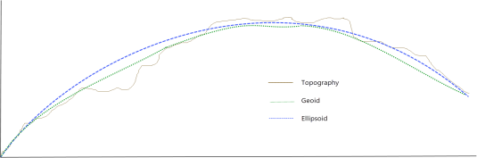
Earth is nearly an oblate ellipsoid, but not an exact ellipsoid – deviations from this shape are continuously evaluated. The shape is known as the Geoid, which is this undulating (by no more than ±100 m) shape that the Earth assumed if it where all measured at sea level. Two geometric constants suffice to define the ellipsoid: the major axis and the flattening. There are numerous principal ellipsoids used in different parts of the globe because the curvature of the Earth is not uniform due to the gravity field.

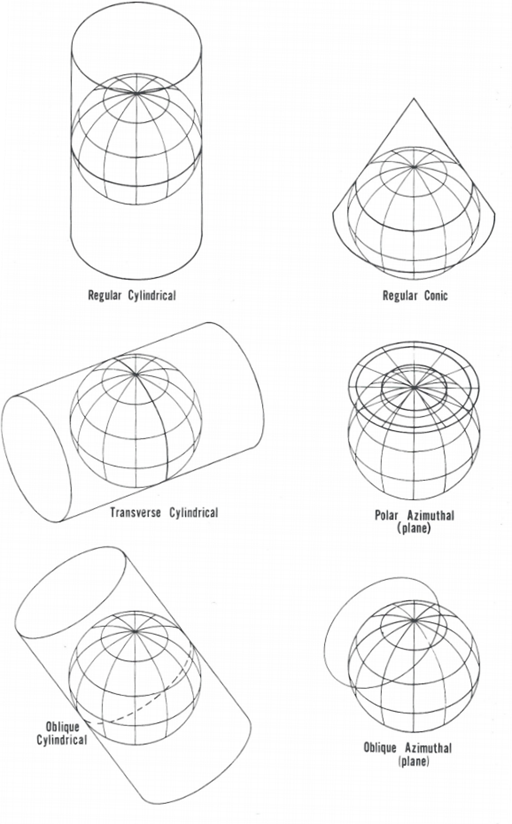
Figure 1 - Projection of the Earth onto the three major surfaces. In a few cases, projection is geometric, but in most cases the projection is mathematical to achieve certain features.

Local Datum Transform

It is important to understand that the LDT is not really part of a coordinate system definition. Stating that coordinates are located on a specific datum effectively defines the coordinate system. The LDT can be thought of as information that a coordinate transformation engine can use if it must transform coordinates across datums. In other words, you are saying “If you must transform these coordinates to another datum, I suggest you use this LDT to convert these coordinates to WGS 84 then to the target coordinate system.” Further, the LDT is not an exact transformation. It is an approximation with an accuracy that depends on the method used, the size of the area for which the LDT applies (usually the larger the area, the less accurate the transformation), and the variability of the shape of the geoid in the region being transformed (more mountainous regions have more geoid variability).

Local datum transforms are listed in the file “ldatum.csv”, which is the list used by this dialog. This list organizes the local datum transforms by area. The local datum EPSG name is referenced in the “Datum_trf” column of this file, and the “datumtrf.csv” file contains the actual local datum transform parameters. If you add your own custom local datum, it must be added to both files. The datum.csv file also contains a column for “Datum_trf”, which indicates the default LDT that will be used for that datum if one is not explicitly selected when defining a coordinate system.

Each local datum transform has an associated datum (such as NAD27). If you choose a local datum transform that is for a datum different from the one selected previously, the datum will be changed. This is allowed, but under normal circumstances it means that there is probably something wrong about the coordinate system you are using. Changing the datum should therefore only be done with caution and an understanding of datum issues.

Understanding Local Datums

Local datum transforms are used to convert coordinates between different map datums. For example, a local datum transform is required to convert longitude, latitude coordinates on the WGS 84 datum to longitude, latitude coordinates on the NAD27 (North American Datum 1927). The difference in location that arises between map datums can be up to several hundred meters.

The key to understanding local datum transforms is an understanding of the geoid and its relationship to a datum. The Geoid is the actual surface of the earth at mean sea level, which is everywhere normal to the earth’s gravitational force. Because of local and regional variations in the earth’s gravity field, the Geoid is not a perfect mathematical form, but rather it has local variations as illustrated in the following diagram (from Verhoogan, John, Francis J. Turner, Lionel E. Weiss, Clyde Wahrhaftig, William S. Fyfe (1970), The Earth, Holt, Rinehart and Winston, Inc., New York.):

 

A datum defines the earth surface on which maps are based when mapping a specific region of the world. Older datums such as NAD27 are based on the Geoid, while newer datums such as WGS84 and NAD83 are based on a spheroid surface. For geoid based datums, a spheroid (also called an ellipsoid) is used to approximate the geoid for the region of the earth mapped using that datum. A spheroid is an ellipse rotated about its shorter axis, which is what the geoid would be if the mass of the earth were uniformly distributed. A datum name implies an ellipsoid (described by the major axis and flattening), the prime meridian (location of 0 longitude, normally Greenwich England), and for geoid based datums, a tie point, which is the location on the earth at which the ellipsoid and the geoid are the same for the region that the datum is used. The ellipsoid and tie point are chosen such that the differences between the surface of the ellipsoid and the geoid are minimized.

Most common mapping operations within the same datum are only concerned with the ellipsoid, which is why an ellipsoid name is often used interchangeably with a datum name. Also, many datums share the same ellipsoid. This has led to the unfortunately common use of different datum names to describe the same area. For example, NAD83 and WGS 84 are both commonly used in North America, Adindan and Arc 1960 are commonly interchanged in North-East Africa, Corrego Alegre and Chua in Brazil, and there are many more examples.

With the advent of satellites and later the Global Positioning System, it became necessary to define datums tied to the gravitational centre of the earth (as opposed to being tied to a location on the earth’s surface). Such datums are called geocentric, and the most common example is WGS 84. Most of the difference between an earth surface tied datum and a geocentric datum can be described by a shift in the location of the centre of the ellipsoid (the assumed earth centre). However, there can also be a small rotation difference caused by differences in the direction of North, and a scale factor caused by differences between the elevation of the tie point and mean sea level. Further, local perturbations of the geoid that result from local gravity variations within a datum will produce additional “residual” differences.

To convert between datums requires knowledge about all aspects of both datums (the ellipsoids, prime meridians, and the local perturbations of the geoid). There are a number of methods used to transform coordinates between datums (see https://epsg.org/), although in practice, the following two methods supported in Oasis montaj are the most commonly used:

1. Simple Shift

The most familiar method is an earth centre shift, rotation and scale, commonly referred to as the Bursa Wolf 7-parameter transform (parameters are X,Y,Z offsets, X,Y,Z rotations and a scale factor). The Molodenski transform is a simplification that deals with three parameters only (X,Y,Z offsets). These transforms are only close approximations to the true perturbations, and datums that cover a large region often require a number of different "local" definitions. As an example, the NAD27 datum has at least six different transforms to WGS 84.

The 7-parameter transform matrix translation equation is:

Where:

dX, dY, dZ = translation parameters, specified in metres (m)

Rx ,Ry, Rz = rotation parameters, specified in arc-seconds (")

Scale = scale difference, specified in parts per million (ppm)

The Bursa Wolf transform is supported in Oasis montaj. Parameters of the transform are listed in the file “datumtrf.csv” for different local datums, and the file “ldatum.csv” contains a reference list based on the common area of use for each datum transform. The transform is applied by first translating to coordinates from the source datum to WGS 84, and then from WGS 84 to the required datum.

It is important to note that although the translation of elevations between datums using the 1-parameter transform is possible, it is only accurate for ellipsoid-based datums such as WGS85 and NAD83. Elevations transformed in this way from geoid based datums such as NAD27 are not accurate. See the note below on “Elevations”.

2. Correction Grid

Some national mapping agencies have carefully measured accurate “residual” differences across a datum. This has been done by measuring the differences between local map coordinates and WGS 84 at numerous locations on the datum. Such differences are described by correction "grids", which contain longitude, latitude and elevation shifts as a function of location. Examples are NADCON in the US and NTv2 in Canada, both of which are supported in Oasis montaj (NTv2 is a 20-minute approximation of the full NTv2 transform). Note that NADCON and NTv2 are not accurately defined for off-shore areas and should not be used for off-shore mapping purposes. In Oasis, the residual correction grids are stored as compressed look-up tables in files with extension “.ll2” in the Geosoft directory. The name of the table is found in the square brackets that are part of the local datum transform name. For example, the lookup tables for local datum transform “*NAD27 NTv2 (20 min) [NTv2]” are found in the file “NTv2.ll2”. In future, as more correction grid models are defined, they will be added to the model list.

Note that Bursa Wolf transforms are very much faster than NADCON or NTv2 and will normally be accurate to the sub-metre level for local regions.

Elevations

The Geosoft coordinate system functions also support the conversion of elevations between datums, although the use of the 7-parameter transform is not considered accurate for elevation translations to or from geoid-based datums. In version 5.1.0, we introduced support for geoid grid models to be added to local datum transforms based on table lookups. The Geoid99 model for translating elevations between NAD83 and NAD27 (sampled at a 4-minute interval) is included as part of the Geosoft NADCON model, and we intend to add other geoid models that become publicly available in the future.

Note that geoid elevation models are described in grid files located in your ".../Oasis montaj/etc" directory. The geoid99.grd is a grid of the NAD27 Geoid relative to the NAD83 ellipsoid. You can use geoid grids to directly look-up corrections for special applications such as correcting WGS 84 elevation to the geoid for gravity corrections.

rX,rY,rZ

Rotations in arc-seconds (arc-second=1/3600 of a degree) to be added to a geocentric Cartesian coordinate point vector in the projection to produce a WGS 84 geocentric Cartesian coordinate vector. The sign convention is such that a positive rotation about an axis is defined as a clockwise rotation of the position vector when viewed from the positive direction of the axis. A positive rotation about the Z axis (Rz) will result in a larger longitude. Most transforms (all Molodenski based projections) will use “0,0,0”.

Scale

The scale correction to be multiplied by the geocentric Cartesian coordinate in the map projection to obtain the correct scale in WGS 84 coordinates. This scale is expressed in ppm so that the actual scale is (1 + scale/1,000,000). For example, “2.25” represents a scale factor of 1.00000225.

Datum Definition Table

The projection information is maintained in the following set of CSV files in the "csv" directory:

area_of_use.csv	Table of projected coordinate systems by their area of use.
datum.csv	Table of EPSG compliant datums. This table includes MapInfo datum numbers, ESRI names, the area of use, the Geoid model, and the prime meridian for each datum.
datumtrf.csv	Table of local datum transforms parameters.
ldatum.csv	Table of local datum transforms by area-of-use.
Datum_alias.csv	Alternate aliases for datum transforms.
ellipsoid.csv	Table of ellipsoid parameters.
ipj_pcs.csv	Table of known projected coordinate systems. This table is not directly used by the projection libraries, but it can be used as a reference by GX’s that are constructing projections, and it is used to resolve the datum and projection given an EPSG projected coordinate system code.
ESRI_CS.csv	Table of ESRI standard transforms.
mapinfo.csv	Table of MapInfo transforms.
transform.csv	Table of map transform methods and parameters. New projection methods will be added to this file.
units.csv	Table of units and factors to convert units to metres.

GDA94 and GDA2020

The GDA2020 projection is a two-step projection: first the data is projected to GDA94, then transformed from GDA94 to GDA2020.

There are two 2D national transformation grids developed by ICSM (Intergovernmental Committee on Surveying and Mapping):

• Conformal: simply a grid version of the 7 parameter similarity (Helmert) transformation: the basic difference between GDA94 and GDA2020 coordinates primarily due to plate tectonic movement (approximately 1.7m NNE over 26 years).
• Conformal + Distortion: incorporates the conformal 7 parameter transformation plus localised and regional distortion revealed by incorporating coordinates on ground survey control networks across the nation.
The distortion component refers to the non-conformal attributes realized from irregular ground movement since GDA94 was established. These effects vary in magnitude and direction around the country and can be as large as 1.5 metres. By applying the distortion grid to transform GDA94 to GDA2020, the localized distortion is removed up to 0.3 metres horizontally.

These transformation grids are available for download from the ICSM GitHub transformation grids repository. For further details on GDA94 ⇔ GDA2020 transformation, go to the ICSM Transformation grids page.

Ordnance Survey Grid Transformation in Great Britain OSTN15 NTv2

All Ordnance Survey mapping relates to a coordinate reference system known as OSGB36 (the “National Grid” – EPSG code 27700). This, in its “native” form OSTN15 consists of a 700 km by 1,250 km square grid of translation vectors at 1km resolution.

Transformation parameters at a particular point are computed via bi-linear interpolation from the parameters at the corners of the km square within which the point falls.

The native direction is ETRS89 to OSGB36. ETRS89 is a precise version of the better known WGS84 (EPSG code 4326) coordinate reference system optimised for use in Europe; however, for most purposes it can be considered equivalent to WGS84.

Transformation type Estimation method Graticule resolution Grid interpolation Accuracy Extent

Interpolation from graticule of latitude and longitude shifts (in seconds) Bi-linear interpolation from native OSTN15 1km grid 30” in latitude, 60” in longitude Bi-linear 0. m (RMS) with respect to OSGB36 primary, secondary and tertiary triangulation monuments, and 0.001m with respect to native 1km grid version of OSTN15 SW corner N49°, W9°; NE corner N61°, E2°. 12° North-South, 11° East-West.

The NTv2 transformation grids are available for download from the Ordnance Survey site OSTN15 and OSGM15 for developers: click on the NTv2 format files (28MB) link to download a zip archive that contains both text and binary NTv2 format files for OSTN15, sample files for testing, and a user guide.
For further details, read the file "OSTN15 NTV2 TRANSFORMATION Data Format and User Guide".

Reference