Tau Calculation
Use the Tau Calculation option to calculate and save an array of running Tau constant values.
Tau Calculation dialog options
|
EM decay channel
|
Input EM array channel (dB/dt or B-field) to calculate Tau constants for. Only arrays with assigned time gates will be displayed in the drop-down list.
Script Parameters: EM_TAU_CALCULATION.SENSOR_CHANNEL
|
|
Noise level
|
All values in the above EM array channel above this threshold will be used to calculate Tau values. Values below this threshold will be ignored.
The default is set to 0.001. Click on the calculator button to reset the default to the Standard Deviation or the last valid channel x10.
Script Parameters: EM_TAU_CALCULATION.NOISE_LEVEL
|
|
Line selection
|
You have the option to calculate Tau constants for the Current line, Selected lines or All lines.
Script Parameters: EM_TAU_CALCULATION.LINE_SELECTION [D – Displayed, S- Selected, A- All]
|
|
Tau channel
|
Base Name of the output Tau constant array channel(s). The individual Tau values calculated on the sliding windows are saved in an array named TauChannel_Tau# where # is the number of consecutive points to fit. Multiple sliding window sizes can be specified at once (see Number of points to fit) in which case multiple Tau array channels will be saved appended by the length of the sliding window.
These arrays are of the same dimension as the input EM array. Elements of the array for which Tau constants are not calculated are filled with dummies
Script Parameters: EM_TAU_CALCULATION.TAU_CHANNEL
|
|
Fit error channel prefix
|
Prefix of the array(s) containing the fit errors for the sliding Tau windows. Tau# is appended to the array name where # is the number of consecutive points to fit. The number of output channels is set by the entry Number of points to fit.
The fit error array(s) have the same dimension as the Tau channel.
Script Parameters: EM_TAU_CALCULATION. MISFIT_CHANNEL
|
|
Window index channel prefix
|
Prefix of the channel(s) containing the array indices of the last EM gate for which a Tau constant has been calculated. Tau# is appended to the array name where # is the number of consecutive points to fit.
These arrays have the same dimension as the Tau channel.
Script Parameters: EM_TAU_CALCULATION.LAST_ELEMENT_CHANNEL
|
|
Save Tau estimate
|
If checked a scalar Tau is also saved and is set to the value of the highest calculated Tau of all calculated Tau arrays. This channel is named after the Tau channel entry.
Script Parameters: EM_TAU_CALCULATION.SCALAR_TAU
|
|
Tau estimate element channel
|
Channel containing the index of the best Tau estimate for that array. This is an optional entry. If left blank no index channel(s) are produced. If provided only rows for which a valid taw has been calculated will be populated.
Script Parameters: EM_TAU_CALCULATION.TAU_ESTIMATE_ELEMENT
|
[More]
|
Boundary Conditions
|
|
Number of points to fit
|
The Tau constants are calculated using a sliding window along the EM array. Specify the number of consecutive EM array elements in the window for calculating Tau constants. You can provide a comma separate list of consecutive array elements as a list of increasing odd values (i.e. 5,7,9). Taus will be calculated for all segment lengths and saved in the database. The basename of the output channels will be appended with _# where # is the number of consecutive elements in the array.
See Application Notes for further details.
Script Parameters: EM_TAU_CALCULATION. TREND_WINDOWS
|
|
Minimum Tau
|
All calculated Tau values below this threshold are either set to dummy or to this limiting threshold.
Script Parameters: EM_TAU_CALCULATION. MIN_TAU
|
|
Maximum Tau
|
All calculated Tau values above this threshold are either set to dummy or to this limiting threshold.
Script Parameters: EM_TAU_CALCULATION. MAX_TAU
|
|
Outside range
|
Specify how to set the Tau values outside the specified range above. Should they be set to the limiting value or simply dummied out.
Script Parameters: EM_TAU_CALCULATION. OUTSIDE_RANGE [0- set to dummy, 1- set to limiting threshold]
|
Time Windows
|
|
Time window selection
|
You can specify which time gates (elements of the array) to use for the Tau calculation. By default, all gates will be used. Alternatively, you can specify the range of time gates by setting the minimum and maximum time gate values, or manually check/uncheck the desired time gates.
Script Parameters: EM_TAU_CALCULATION. WINDOW_SELECTION [0-All, 1-Range, 2- Manual]
|
|
Minimum/Maximum time
|
These 2 entries are activated only if you have selected the Outside range option above to enable you to define the range.
Script Parameters: EM_TAU_CALCULATION.MAX_TIME
|
Application Notes
The rate of decay of the transient EM data is an indicator of the conductivity/geometry of the subsurface, hence it is used to discriminate conductors from overburden. The rate of decay is directly related on the conductance regardless of depth. The decay voltage at the receiver is proportional to the time rate of change of the secondary magnetic field. Conductive targets have a relatively low initial value and decay relatively slowly. Resistive material have a relatively high initial value and decay fast. We can thus formulate that the decay voltage is proportional to an exponential decay term as a function of time (t) and controlled by a Constant Ʈ that is an indicator of the conductance as:
B-Field is proportional to 
EM instrumentation measures the variation over time dB/dt of this field:
dB/dt is proportional to 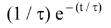
Conductive material will yield large Ʈ values while resistive material yields small Ʈ values. Gridded Tau values could thus be a useful interpretation tool.
This tool calculates a series of Ʈ values using a sliding approach along the EM decay array (highlighted with orange boxes in the illustration below). The tool calculates a series of Ʈ constants for consecutive N points by fitting the exponential component e-t/τ. The sliding window moves by one element at a time. The calculated Ʈ is saved at the midpoint of the sliding window (indicated with grey arrows for each window in the illustration below). If an even number of consecutive points has been chosen, then the fitted Ʈ is saved at the relative element N/2.
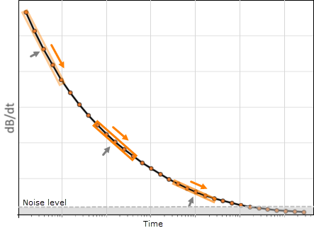
The sliding approach terminates when the EM decay curve reaches the noise threshold, and the remainder elements of the Ʈ channel are set to dummy. The last element (time gate) used for calculating Ʈ is saved in the Last element channel.
Depending on the targeted intent, you could proceed to extract, and/or filter, and/or interpolate, then grid time slices of Ʈ. You can also apply a math expression to extract the latest Ʈ or the largest Ʈ.
