Matched Filtering
Use the 2D Filtering > Matched Filtering menu option (geogxnet.dll(Geosoft.GX.FFT2D.MatchedFiltering;Run)*) to interactively define a set of matched filters.
The matched filters are tapered bandpass filters that collectively cover the entire spectrum. The first filter is a low pass, the last filter is a high pass and the in-between filters are bandpass filters.
Matched Filtering dialog options
Spectrum Pane
|
At the onset, this pane is empty. As soon as you select an Input grid,the interactive spectrum graph displays the input grid’s radially averaged power spectrum as a function of wavenumbers. This spectrum is plotted in black. Once you define your first depth, two filters with distinct colours are displayed on the graph, and the filtered spectrum in focus is displayed in red. If more depths are specified, the corresponding filters and output spectra acquire other distinct colours. A legend along the bottom of the graph identifies them.
The range of the abscissa spans from 0 to ½ cell size. For convenience and because you provide the parameters in wavelengths rather than wavenumbers, you can toggle between wave numbers and wavelength (1/wavenumber). However, this does not affect the graph.
In order to allow a finer control in the longer wavelengths (or lower wavenumbers), the minimum wavelength can be adjusted up to a factor of 10. You can change the range by editing the value at the right end of the abscissa.
The ordinate is annotated with the logarithm of the power spectrum on the left and the range of the filter coefficients on the right. You can change the range of the power spectrum by editing the end values of the ordinate.
When you change the graph range, the reset button ( ), located at the bottom left of the graph, becomes active and allows you to return to the initial data range. ), located at the bottom left of the graph, becomes active and allows you to return to the initial data range.
The Spectrum pane is resizable in both directions. To resize the pane, grab the horizontal or vertical grip by holding the left mouse button down on the grip (Figure 1).
|
Filter Definition
This is where you select the input grid and define the matched filters. You can define a maximum of four equivalent depths. N depths produce N+1 separate bandpass filters.
When you specify a depth and press <Enter>, all the other panes are updated to reflect the effect of the new depth on the spectrum and output grid.
|
|
Input grid
|
The magnetic input grid to which the matched filters will be applied.
Pre-processing (trend, expansion and fill) is applied prior to filtering; see Application Notes below for more details.
|
|
Data type
|
Select Magnetics if the input grid provided is a pole reduced magnetic grid. This is the default option.
You should first pole reduce the magnetic grid, as picking of the slopes for depth determination should be made on pole reduced magnetic grids.
Select Gravity if your grid is a gravity grid. In this case, the spectrum graph is first divided by the wavenumber in order to obtain the equivalent magnetic spectrum. This is the spectrum that will be displayed and from which the depths will be selected and calculated.
Note that the resulting filters will be applied to the input gravity data.
|
|
Output grid prefix
|
Specify a prefix for the output filtered grid(s). You will have as many output grids as defined filters/layers. The default prefix name is set to matched; however, you can override the default.
|
|
Number of depths
|
Enter a depth number (or use the up and down arrow buttons). You will be prompted to enter depth values according to the number of depths entered. A maximum of four depths can be specified.
The correlation between depth and central wavenumber is depth = gradient/4π. The gradient is obtained from the log radial average spectrum. These depths are also calculated in 2D Filtering > Display Radial Spectrum.
|
|
Window width
|
Enter a number or use the up and down arrow buttons. The window width should be an odd number between 3 and half the spectrum length. The default is set to 1/10th of the spectrum length.
Since generally the radial spectrum is noisy, to calculate the equivalent depth along the radial spectrum at the cursor location, a least square fitting is first applied to the specified window width number of points centered on the cursor location; then the equivalent depth is the inverse of the slope of the locally fitted line.
|
|
Depth #
|
After entering a value, press the <Enter> key, and the spectra and associated output preview image will automatically update.
Click on the  icon to the right of the Depth # field to interactively select the filter depth on the spectrum graph. icon to the right of the Depth # field to interactively select the filter depth on the spectrum graph.
|
Preview Pane
The preview pane offers an interactive view of both the original grid and the filtered grid(s). The images in the two preview windows are linked and the cursor location is tracked. The most recent colour table assigned to the input grid is used to display the images in the preview pane.
The preview pane is resizable; grab the grip at the bottom right of the pane to resize the pane.
|
|
Original grid
|
At the onset, this pane is empty. When you provide an Input grid, it is displayed in this pane.
|
|
Output grid(s)
|
This is an interactive image view of your output filtered grid(s).
At the onset, this pane is empty. When you define depth(s), the output depth grids are calculated and can be viewed in this pane. You can preview one output grid at a time. The selected Preview output depth layer is the one displayed in this pane.
|
|
[Zoom]
|
To zoom into a location on both grids, click the Select and zoom to an area of interest (  ) button.
Note that your cursor changes to a select mode when it crosses either the Original grid or the Filtered grid(s) windows. ) button.
Note that your cursor changes to a select mode when it crosses either the Original grid or the Filtered grid(s) windows.
Using your cursor, draw a box around the desired area,
then click inside the boxed area to zoom to the selected location. Click the Show entire data extent ( ) button to return your zoomed images to the original full size. ) button to return your zoomed images to the original full size.
|
Application Notes
The yellow asterisk (  ) indicates a required parameter.
Up to five filters (four equivalent depth layers) can be defined.
The preview pane windows enable you to view both your original grid and your resultant filtered grid(s). As you interactively modify your filters, the results can be immediately viewed in the preview output window.
Pre-processing:
Similar to MAGMAP Filtering, the input grid must undergo pre-processing prior to wavenumber domain filtering. This stage consists of the following steps:
-
Using the edge points of the input grid, the first order trend is calculated and removed from the grid.
-
Next, using the Winograd algorithm (see MAGMAP Filtering), the grid is expanded by approximately 10% to a square.
-
Finally, using the Maximum Entropy extrapolation method and ensuring data continuity across opposite edges, the grid is filled.
Since the Matched Filtering tool is built on the base of MAGMAP, it inherits the MAGMAP settings. As a result, the above are the MAGMAP pre-processing defaults. If you have executed MAGMAP prior to running the Matched Filtering tool, and in the course of doing so, you modified the pre-processing parameters, the Matched Filtering tool inherits these latest MAGMAP pre-processing parameters.
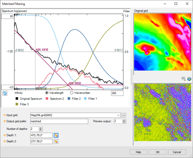
Figure 1: Matched Filtering
To allow you to better visualize the panes, maximize and minimize buttons are located on the dialog's title bar, while the Help button has been placed alongside the OK and Cancel buttons at the bottom of the dialog.
*The GX tool will search in the "...\Geosoft\Desktop Applications \gx" folder. The GX.Net tools, however, are embedded in the geogxnet.dll located in the "...\Geosoft\Desktop Applications \bin" folder. If running this GX interactively, bypassing the menu, first change the folder to point to the "bin" folder, then supply the GX.Net tool in the specified format.
References
- [1] D. R. Cowan, "Separation Filtering Applied to Aeromagnetic Data", Exploration Geophysics, vol. 24, no. 3-4 (1993), pp. 429-436.
- [2] Jeffrey D. Phillips, "Designing matched bandpass and azimuthal filters for the separation of potential-field anomalies by source region and source type", ASEG Extended Abstracts, vol. 2001, no. 1 (2001), pp. 1-4.
- [2] P. J. Gunn, "Linear Transformations of Gravity and Magnetic Fields", Geophysical Prospecting, vol. 23, no. 2 (1975), pp. 300-312. DOI: https://doi.org/10.1111/j.1365-2478.1975.tb01530.x
