MAGMAP Filtering

Use the 2D Filtering > MAGMAP Filtering option (geogxnet.dll(Geosoft.GX.FFT2D.MAGMAPFiltering;Run)*) to apply common Fourier domain filters to gridded data.

MAGMAP Filtering dialog options

Application Notes

1. Overview

Fourier Domain filtering (often referred to as FFT Filtering) provided by MAGMAP Filtering enables the following kinds of processes to be applied to 2-D gridded data:

Potential Field Filters

• Reduction of magnetic data to the magnetic pole or magnetic equator.

• Differential reduction of magnetic data to pole.

• Transform from pole to any inclination/declination.

• First/second/nth vertical derivatives.

• Upward and downward continuations to any horizontal surface.

• Apparent magnetic susceptibility maps from magnetic field.

• Apparent density maps from residual gravity field.

• Optimum Wiener depth filter.

• Conversion between different directional components of the field.

General Purpose Filters

• Six different regional/residual separation filters.

• De-corrugation and directional filters.

• First/second/nth horizontal derivatives.

This is not a comprehensive list. For more filters, see the links at the bottom of this document.

2. MAGMAP Processing System

For the sake of mathematical convenience and speed, MAGMAP Filtering applies filters in the wavenumber or Fourier domain. This requires several steps:

1. Pre-processing: the original space domain grid is trend removed, expanded and filled. The fill routine maintains data continuity on opposite edges of the grid.
2. Transformation: the space domain data is transformed to Fourier domain.
3. Filtering: filter operators are applied.
4. Inverse transformation: the filtered data is transformed back to space domain.
5. Post-processing: the filtered grid is masked to the same footprint as the original grid; the regional trend is replaced.

Following are descriptions of each of the processing steps.

Pre-processing (creates _prp.grd)

1. The background trend is removed from the gridded data. The trend can be a DC shift (0^th order), a linear trend (1^st order) or a very long regional trend emulated with the 2^nd or 3^rd order trend. This step reduces the potential of introducing high power long wavelength into the data through the process of filling the grid while maintaining periodicity. If the background is around zero, the extrapolated data will reside within the spectrum of the real data and thus the outcome will not suffer from the artifacts of the Digital Fourier Domain processing.

2. The trend removed grid is then expanded in order to prepare it for the Fourier transform process. MAGMAP uses either the Cooley-Tukey or the Winograd algorithm. The Cooley-Tukey algorithm requires that the dimensions of the input grid be a power of 2 (i.e. 2, 4, 8, 16, 32,...,1024, 2048, 4096). It is preferable to expand the grid as little as possible while maintaining continuity and periodicity. To circumvent the dilemma of the increasing difference of successive powers of 2, Winograd came up with an alternative algorithm supporting more frequent permissible dimensions. The Winograd dimensions are (2, 4, 6, 8, 10, 12, 14, 16, 18, 20, 24, 28,..., 1008, 1260, 1680, 2520, 5040).

3. The dummies in the expanded grid are then filled using one of the three available methods such that the grid is smoothly periodic across opposite edges. If you think of the grid as a single square/rectangular tile and copies of the tiles are laid out edge to edge, the grid pattern should smoothly match from tile to tile. If the matches were not smooth, an effective 'step' function would be introduced at the edge of each grid - this would cause serious side effects in the data when transformed back to space domain.

   • The Maximum entropy method (MEM) uses a segment of the real data to predict the extension. The principle of maximum entropy postulates that given a set of known data, the probability distribution that best represents it is one that has the largest entropy or uncertainty. MEM uses this stipulation to calculated coefficients that are convolved with the real segment in order to predict the expended segment. This method is the default method and behaves properly with most geophysical datasets.
   • The Inverse distance is a method that quickly attenuates the extrapolated data and is most useful when the real data along the edge has a high frequency high amplitude nature. This is the least used method.
   • The Multi-trend expansion method uses the NSI gridding algorithm developed by Tomas Naprstek and Richard Smith of Laurentian University ². Use this method if your data contains thin linear features that span across multiple survey lines and the data does not contain a predominant strike direction.

The expanded and filled grid is saved in the working folder. It retains the base name of the input grid and is appended by _prp.

Forward Fourier Transform (creates _trn.grd)

The expanded/filled grid is transformed to the Fourier domain where the filters are applied. In the field of digital signal processing these two domains are referred to as time and frequency domains; the units of the former is “t” and the latter “t^-1”. By analogy since geophysical data has a spatial attribution, in order to apply Fourier domain filtering, it is converted from space (m) to wavenumber (m^-1) domain.

In one dimension, the Fourier transform is represented with the integral:

H(υ)=

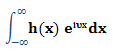
Where: 

              x is the distance variable

              υ is the wavenumber variable

              h(x) represents the signal in space domain

              H(υ) represents the signal in wavenumber domain

Since the operation is performed in a two dimensional space, the space domain variables are x and y, and the wavenumber domain equivalents are u and v.

Expressing the transformation in 2 dimensions:

H(υ,ν)=

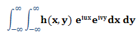
Where: 

             h(x,y) represents the signal in space domain

             H(υ,ν) represents the signal in wavenumber domain

The transformed grid retains the base name of the input grid and is appended by _trn.

For practical reasons, the transform grid is saved in the Geosoft grid format, the axis of which are the wavenumber domain υ & ν. See Display 2D Spectrum for further description.

Output TRN (_trn.grd) and PRP (_prp.grd) Grids

By default, the TRN grid and the PRP grid will be created in the current working directory. This location can be changed in a script by setting the parameters:

MAGMAP1.OUTTRNGRD="full path to grid file.ext(qual)"

MAGMAP1.OUTPRPGRD=" full path to grid file.ext(qual)"

Radial Energy Spectrum (creates *.spc)

Once the Forward Fourier Transform is created, the radially averaged energy spectrum is also calculated. This data is saved in an ASCII file constructed using the input file base name and the extension *.spc. The format of this file (example below) consists of:

• header containing:
• the averaged energy value over the entire transform.
• the labels of the five columns that follow.
• five numeric columns of data.

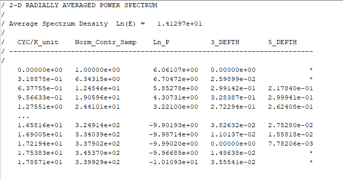
The 2D energy at each υ & ν point in the wavenumber domain consists of the square sum of its real and imaginary components. The radial energy spectrum that follows (3^rd column) is normalized by the transform averaged energy listed in the header.

The 1^st data column, CYC/K_unit, contains the radial increment in the wavenumber domain.

The 2^nd data column, Norm_Contr_SAMP, represents the circumference at the radial increment, normalized by the radial increment. This is an indicator of the relative number of contributing elements.

The 3^rd data column, Ln_P, lists the averaged energy of all elements at the wavenumber radius (1^st column). The energy is normalized by subtracting the log of the average spectral density.

The 3-DEPTH and 5-DEPTH columns are ensemble magnetic depth estimates based on 3- and 5-point averages of the slope of the energy spectrum³.

The depth to a statistical ensemble of sources is determined by the following expression:

h = −s/4π

Where:

h is depth

s is the slope of the log (energy) spectrum

The above estimates can be used as a rough guide to the depth of magnetic source populations.

Define Filters

You can define the filters in the interactive MAGMAP Filter Design window.

Multiple filters can be applied concurrently. The Fourier domain filters are commutative and the order in which they are supplied is immaterial. You will be prompted for additional parameters according to each filter’s requirements. For example band-pass filters will prompt the user to specify two cutoff wavelengths. This information is saved in the specified filter control file (*.con).

Filtering

The filters are defined and applied to the Fourier transformed grid.

H(υ,ν)= H(υ,ν) . F(υ,ν)

Where:  F(υ,ν) represents the two dimensional filter.

Note that in order to filter the data, for each element (υ,ν) of the grid, a single multiplication is performed.

Inverse Fourier Transform

The filtered grid is transformed from the wavenumber domain back to the space domain through the following formula:

h(x,y)=

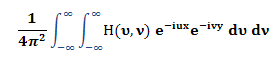
Post-processing

1. This step uses Boolean operations to match the filtered grid to the original input grid size. For example, if our original input grid was 29x15, and it had been expanded to 32x16 using the Cooley-Tukey method in the pre-processing stage, then it is now deflated back to 29x15.

2. The trend is then added back into the grid.

3. Size Consideration

There are no software limits on the size of the grid to filter. However, in order to successfully filter a very large grid, a few considerations must be made:

1. Do not run other memory intensive operations at the same time with MAGMAP Filtering.
2. Use the Maximum entropy method to fill the expanded grid.
3. Ensure that the size of your expanded grid is reasonably smaller than the RAM available: nX *nY * 8 << available RAM.

References

- [1] S. Winograd, "On Computing the Discrete Fourier Transform", Mathematics of Computation, vol. 32, no. 141 (January 1978), pp. 175-199
- [2] T. Naprstek and R.S. Smith, "A new method for interpolating linear features in aeromagnetic data", GEOPHYSICS, vol. 84, no. 3, pp. JM15-JM24, 2019
- [3] A. Spector, "Statistical Analysis of Aeromagnetic Data", Thesis/dissertation, University of Toronto, chapter 5, section 2 (1968)