
MAGMAP Filter Design
Use the interactive filter design dialog to define the Fourier domain filters and to interactively preview the original grid and the filtered grid(s). If the filter file provided in the MAGMAP Filtering dialog is a pre-existing filter control file (*.con) , the filter values stored in that file will be loaded by default in this dialog. Filter parameters can then be interactively modified to obtain the best results for your data.
The preview pane windows enable you to view both your original grid and your resultant filtered grid(s). As you interactively modify your filter parameters, the results can be immediately viewed in the Filtered Grid window.
MAGMAP Filtering | Create/Edit Filter dialog options
 ), located at the bottom left of the graph, becomes active and allows you to return to the initial data range.
 ) button located at the bottom right of the pane. Each filter has its own specific parameters. The
  ), or by entering the values directly in the parameter fields (
 ). After entering a parameter, press the <
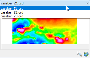
Application Notes
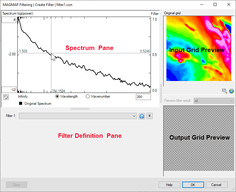
Figure 1: MAGMAP - Interactive filter layout
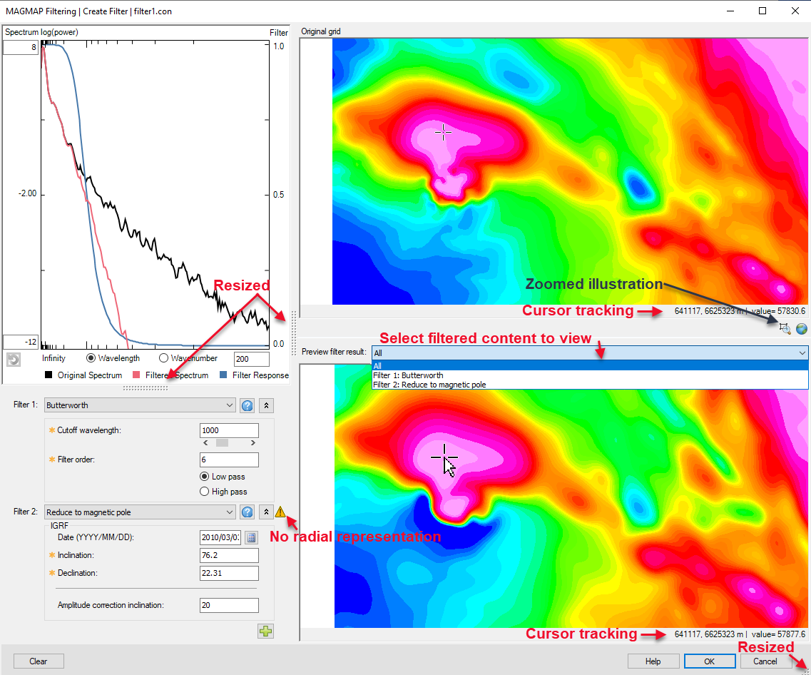
Figure 2: MAGMAP - Interactive definition of filters
Grid Size Consideration
If the input grid is very large, the interactive refresh of the graph/images in the MAGMAP filter window could be slow. To circumvent the potential delay, when the input grid is larger than 2048 cells in either dimension, the grid is decimated to dimensions less than 2048. The decimated grid is saved in the working folder and is reused in subsequent invocations of the MAGMAP interactive filter. If you delete the preview grid, next time you run MAGMAP it will be recreated. The decimated grid inherits the base name of the input grid appended by "_preview". Its transform inherits the base name of the input grid appended by "_preview_trn". The decimated grid and its transform are only used to produce the graph/images in the Magmap filter window. The final grid is produced using the original grid as input.
Finding Help for a Specific Filter
Once you have selected your filter of interest, the filter information is available by clicking the  button located beside the Filter drop-down or by using one of the links below. Additional information can be found in the
To allow you to better visualize the preview panes, maximize and minimize buttons are located on the dialog's title bar, while the main Help button has been placed alongside the OK and Cancel buttons at the bottom of the dialog.
See Also:
- MAGMAP Filtering
- Define Filters
- Apparent Density Calculation (DENS)
- Apparent Susceptibility Calculation (SUSC)
- Bandpass (BPAS)
- Butterworth (BTWR)
- Butterworth Bandpass (BTWRB )
- Butterworth Notch (BTWRN)
- Conversion Between Field Components (TXYZ)
- Cosine Roll-off (COSN)
- Cosine Roll-off Bandpass (COSNB)
- Derivative in the X, Y, Z Direction (DRVXYZ)
- Differential Reduction to Magnetic Pole (DRTP)
- Directional Cosine (DCOS)
- Directional Pass/Reject (DPAS)
- Downward Continuation (CNDN)
- Gaussian Regional/Residual (GAUS)
- General Radially Symmetric (GNRL)
- Gravity Earth (GFILT)
- High-pass (HPAS)
- Horizontal Integration - X (INTGX)
- Horizontal Integration - Y (INTGY)
- Low-pass (LPAS)
- Notch (NOTCH)
- Pseudo-Gravity (GPSD)
- Reduce to Magnetic Equator (REDE)
- Reduce to Magnetic Pole
- Transform from Magnetic Pole (TRFP)
- Upward Continuation (CNUP)
- Vertical Integration (INTG)
- Wiener Optimum (OPTM)
- 2D Fast Fourier Transform Theory
Got a question? Visit the Seequent forums or Seequent support
© 2023 Seequent, The Bentley Subsurface Company
Privacy | Terms of Use