Display Grid on Map

Use the Grid and Image > Display on Map > Grid menu option (geogxnet.dll(Geosoft.GX.GridUtils.DisplayGrid;Run)*) to place a grid image on a map.

You can display up to four grids or images on a map at once by using one of the composite grid options available.

Display Grid dialog options

Grid name

Select the grid file to display on a map.

For a list of supported grid formats, see the topic Supported Data Formats.

For details on crooked sections, see the topic Crooked Section Grids.

Script Parameter: GRIDIMG1.GRID

Colours

Select the colour scheme for rendering the image of the selected grid. If you mouse over the Colours entry, a tool tip will display the name of the colour table file. To modify the selection, click on the colour entry and then navigate through the scheme categories.

Script Parameter: GRIDIMG1.COLOR

Colour method

Select the colour method as one of the following options: As last displayed, Default, Histogram equalization, Normal distribution, Linear, Log-linear.

The method "As last displayed" will display each grid as it was displayed the last time the grid was viewed, and the colour tables will be ignored.
If the selected colour scheme is an .itr file or a .zon file, the colours are already attributed to data ranges, and this entry remains disabled.

Script Parameter: GRIDIMG1.ZONE [0 – Default (set in the global setting); 1 –Linear; 2 – Normal distribution; 3 – Histogram equalization; 5 – Log-Linear; 6 – As last displayed]

Brightness

The normal brightness is defined at 0. You can change the brightness from -100 (black) to 100 (white) using either the slider bar or by entering an exact value.

Script Parameter: GRIDIMG1.BRIGHTNESS [range: 0 to 100]

Reverse colour distribution

The colour table can be used in reverse order. Check this box to reverse the order of the colour scheme.

For example, the colour table for displaying resistivity data is the inverse of the one used for conductivity. By allowing to reverse the colour table on the fly, the same table can be used to display both.

Script Parameter: GRIDIMG1.REVERSE [0-No | 1 - Yes]

Smoothing

For display purposes, by default, the grid is first interpolated to a smooth image at the screen resolution. If you prefer to honour the grid resolution, leave the Smoothing option unchecked: the image will appear pixelated and the colour will change at the actual grid interval rather than the screen resolution.

Script Parameter: GRIDIMG1.PIXEL [0-No | 1 - Yes]

Shading

Adding a shading effect to the colour grid emphasizes the subtle changes in the data that would otherwise be subdued. Presenting the data shaded is optional.
Check this option to shade the colour grid image. If checked, by default the sun angle is set to an inclination & declination of 45°. You can further customize the sun angle and the shading effect by clicking on the More button and then on the Shading Effect tab.

See the Shading section in the Application Notes for further details.

Script Parameter: GRIDIMG1.SHADOW [0-No | 1 - Yes]

Add colour bar

Check to add a colour bar for this grid on the map.

Script Parameter: GRIDIMG1.COLOUR_BAR [0-No | 1 - Yes]

Location

Specify the location as Default registration (default option) or Fit to an area (user defined - interactive only).

When you place an image or grid on a map, the system assumes you are using the default registration system as defined in the grid or image header. If you want to position the grid interactively, select the option Fit to area; then use the mouse to define a rectangular area on the map and the system will fit the grid (or image) exactly to this area.

Script Parameter: GRIDIMG1.REG ( 0 for default registration from image)

[More]

Data Range

Contour interval

The minimum contour interval for rounding the colour breaks. Provide a suitable number around 1/10 of the standard deviation of the data to generate a similarly coloured image but with rounded colour break values.

Script Parameter: GRIDIMG1.CONTOUR

Minimum value

All grid values below this threshold will be displayed with the lowest colour defined in the table. To reset it to default, click on the calculator button.

Script Parameter: GRIDIMG1.MINIMUM

Maximum value

All grid values above this threshold will be displayed with the highest colour defined in the table. To reset it to the default, click on the calculator button.

Script Parameter: GRIDIMG1.MAXIMUM

Shading Effect

Enabled when the Shading option is checked.

Wet look

The shading effect consists of superimposing on the colour image the grey-scale gradient of an overlapping data grid. This is known as the normal shading effect.
In addition, you could make the colour saturation vary with the sun angle. To enable this mode, check the Wet look box.

The colour table specified is ignored when shading using the "Wet-look (HSV)". Instead, hsvc.tbl and hsvg.tbl are used for the colour and shaded components of the image respectively; see the Application Notes below for more details.

Script Parameter: GRIDIMG1.SHADING_TYPE [0 – Normal, 1 – Wet Look]

Shadow grid name

Select a coinciding grid, such as a topography grid, to generate the shading. If left blank (default), the input grid will be used to generate the shading.

Script Parameter: GRIDIMG1.SHADOW_GRID

Inclination

Illumination inclination. By default inclination is set to 45°.

Script Parameters: GRIDIMG1.INCLINATION

Declination

Illumination declination. By default declination is set to 45°.

Script Parameters: GRIDIMG1.DECLINATION

Vertical scale factor

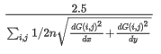
The scale factor to apply in order to balance the shading.

The scale determines how the shading tool interprets the values in your grid. For example, if you use a large scale, you will exaggerate the vertical appearance of your grid and see deep valleys. If you use a very low scale, you will flatten the grid and see very smooth hills.

See the Shading section in the Application Notes for further details.

The default vertical scale factor is set to 2.5 over the mean of the gradient of the input grid.

Where:

n=i*j

i,j -> grid indices

dG/dx & dG/dy -> gradient in X & Y directions

To obtain this value or to reset it, click on the calculator button.

Script Parameters: GRIDIMG1.VERTICAL_SCALE

[New Map]

[Current Map]

Click the New Map button to display a grid on a new map. If the map already exists, you will be prompted to overwrite or provide a different name.

Click the Current Map button to display the grid on the current map.

Script Parameters: GRIDIMG1. NEW [1 - New map, 0- Current map]

Application Notes

Accessing ER Mapper Bands

Oasis montaj enables you to work with a variety of grid and image formats — freely importing them, specifying certain grid parameters (such as specific bands) and exporting them as required. The procedure for accessing (importing) an image by placing it on a map is similar to the method for importing a grid.

The basic mechanism for accessing grids and images is provided through a special technology called DAT. DATs are DLLs that provide interfaces to a variety of image and grid formats. Each DAT has a 3-letter identifier and a number of parameters that can be used to "decorate" the file name when accessing a file for import or export.

For example, to access the third band of a TM image in an ER Mapper image named "CITY.ERS", you would "decorate" the name as follows:

City.ers(ERM;band=3)

The first parameter in the decoration block (inside the parentheses) is always the 3-letter DAT identifier, which you must supply any time you want to specify a decoration. If you do not specify a decoration, the default DAT type is taken from the "DAT Settings" parameter in the Advanced Settings dialog.

You can also specify decorations when exporting grids and images or use decorations to convert them to another format.

For a complete list of decorations currently available for use in the system see the topic XGD DAT Qualifiers.

Colour Tables

To help you navigate through the colour schemes more effectively, the installed colour scheme files (e.g., colour tables (*.tbl) , colour zones (*.zon) , etc.) are organized in subfolders, each defining a category.
In addition, this tool keeps track of three custom categories, and finally you still have access to browse outside of the structured categories.

The colour schemes have been subdivided into the following categories:

System Categories

Geophysics: contains colour tables appropriate for displaying single-entity geophysical data, such as total magnetic intensity, gravity, resistivity, induced polarization.
Topography: contains colour tables that convey the feel of terrain and should be used to display elevation or topography.
Monochromatic: Radiometric data is generally displayed as an overlay of three normalized elements on a single colour map; each element is displayed using gradations on a single colour. All monochromatic tables along with shadow tables are found under this category.
Heat map: Originally devised for depicting financial information and later to display frequency of web page visits, the schemes found under this category lend themselves well to thematic data display.
CET perceptual: The Centre for Exploration Targeting of the School of Earth Sciences at The University of Western Australia has produced a set of perceptual colour schemes that are freely available. For your convenience, we provide them with Oasis montaj.
Perceptually uniform: The perceptual contrast of adjacent colours may vary widely for some colour schemes. The result is that in some sections of the colour scheme, the data variation will be less visually noticeable (dead zone) than in other sections, preventing a proper interpretation. Perceptually uniform colour schemes offer the same visual contrast throughout the colour scheme.
Miscellaneous: Some specialized Oasis montaj extensions trigger the installation of additional colour schemes. In order to easily find them, these schemes are grouped in a separate category labeled "Miscellaneous". This category will only appear if you actually have such extensions.

Contextual Categories

Custom: You may want to access your custom colour tables you have compiled over time. These can be a collection of tables you downloaded from various sources or generated yourself. The recommended location to keep such tables is the %USERPROFILE%\Documents\Geosoft\Desktop Applications \tbl folder. The Custom category points to this folder, which persists across upgrades.
Project directory: You may have custom colour tables specific to your project that you access from your working directory. This category will only appear if you actually have colour tables in your working folder.
Favourite: The colour scheme defined in the General Settings dialog (accessed from the menu Project > Settings > General) is your default colour scheme, and it is explicitly made available under the "Favourite" category.

[Browse...]

Provides the option to navigate outside of the above structure and locate a colour scheme file. In the 'Browse for colour scheme file' dialog, use the buttons to toggle between your working folder (Project Directory), the Oasis montaj program directory (Geosoft Colour Tables), and your default %USERPROFILE% folder (User Colour Tables).

Shading

Colour shaded grids are a valuable interpretation tool to verify gridded data quality as well as to identify structural trends within gridded data.

To display a shaded relief, Oasis montaj creates an auxiliary grid file in the directory where the input grid resides. This grid has the same base name as the input grid followed by the suffix "_s", and it gets created every time you opt to view a shaded grid. If this auxiliary grid file already exists, it is overwritten. After the shadow grid image is created, you can use the Colour Tool to modify the shading parameters interactively.

The stronger the data variation, the shorter the shadows and the faster the progression from dark to light. In addition, the higher the illumination inclination from the horizon, the shorter the progression from dark to light. In order to balance the shading to accommodate a wide range of data distributions and illumination angles, the shadow distribution is widened for strong data variations and high illumination angles through the use of the Vertical scale factor.

The shadow grid is thus calculated using the following equation:

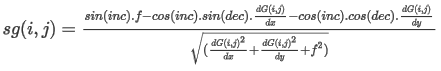
Where:

sg 	-> shadow grid

i,j 	->  i^th row & j^th column grid indices

inc 	-> illumination inclination

dec 	-> illumination declination

f	-> 1/ VerticalScaleFactor

dG(i,j)/dx -> gradient of the i,j grid point in the X directions

dG(i,j)/dy -> gradient of the i,j grid point in the Y directions

HSV

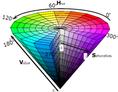The Hue component describes the colour itself in the form of an angle between [0°,360°]. The illustration shows the angular values of the entire colour pallet. For example, red is assigned 0° and cyan is at 180°. To abide to the Geosoft colour table format, colour must be represented with a 1 byte integer, thus the 360 range is scaled to a 255 range. When invoked, the Display Grid tool converts it to the right range on the fly.

The Saturation component is between 0 & 1, where 0 indicates the absence of colour and 1 its full intensity. In the illustration, it is represented by the radius of the circle.

The Value component spans from 0 to 1, where 0 is the darkest (black - at this point the values of H and S are irrelevant), 1 the brightest. In the illustration, it is represented by the vertical component. The S & V components influence the shading and the contrast, which are controlled by the inclination and declination of the sun angle. To abide to the Geosoft colour table format, both the S & V components are also scaled to [0,255], and the Display Grid tool converts them to the right range on the fly.

The colour distribution for a HSV image (1st column of hsvc.tbl) is translated to the 3 RGB components on the fly and scaled for brightness and contrast ( 2nd & 3rd columns of hsvg.tbl) along the sun shadow angle.

Unlike the RGB colour distribution option, the HSV tables are not static tables but generated on the fly, and as a result you can not use the Colour tool to modify it.

*The GX tool will search in the "...\Geosoft\Desktop Applications \gx" folder. The GX.Net tools, however, are embedded in the geogxnet.dll located in the "...\Geosoft\Desktop Applications \bin" folder. If running this GX interactively, bypassing the menu, first change the folder to point to the "bin" folder, then supply the GX.Net tool in the specified format.