Terrain Correction

Use the Gravity > Terrain Corrections >Terrain Correction menu option (geogxnet.dll(Geosoft.GX.Gravity.TerrainCorrection;Run)*) to calculate the gravity terrain effect. The terrain correction is calculated for each station in the database, using a correction area of 2 × correction distance by 2 × correction distance, centered on the station. The results are saved in the output terrain correction channel.

Terrain Correction dialog options

Elevation channel	Select the elevation channel. This is the elevation of the survey instrument relative to the reference datum. The axis is defined as positive above the reference datum. The reference datum is generally, but not necessarily, set to the sea level. Script Parameter: GRTERAIN.ELEVCH
Topography (top of rock) grid	Specify the most detailed grid defining the boundary of the solid rock with air or water. If the survey area spans multiple bodies of water, this grid defines the contact of the solid material with air over bodies of water and the contact of the solid material with air everywhere else. The topography grid must extend beyond the survey area by at least the specified terrain correction distance value. The extent of the topography grid depends on the topographic relief of the area. If there are significant masses or deficiencies of masses in the survey area, they will strongly influence the terrain effect. In such cases, extend the grid further. For relatively flat terrain areas, an additional ~25 km beyond the survey area is generally sufficient. In regions of pronounced topography, extend the grid further—but not beyond 167 km, where Earth curvature has a stronger contribution than the topographic variability. Essentially, surface masses beyond this distance should produce negligible gravitational effects at the survey stations. If the topography grid does not extend at least as far as the correction distance beyond the survey area, the terrain beyond the grid is assumed to reflect on the opposite grid edges of the topography grid out to the correction distance (see Figure 3). Script Parameter: GRTERAIN.DEMGRD
Correction distance	Specify the correction distance. This is the horizontal distance beyond the survey area to be included in terrain effect calculations, and it depends on the degree of topographic relief (refer to the Application Notes for guidance). Script Parameter: GRTERAIN.DIST
Earth density	Specify the density of the earth in grams per cubic centimetre (g/cm³). The default value is 2.67 g/cm³. Script Parameter: GRTERAIN.DENST
Water reference datum	When bodies of water are present within the survey area, you can define the water level using either a constant value or a grid. Select the Constant option if the survey area includes a single body of water or if all bodies of water share the same elevation. Select the Grid option for areas with high topographic relief and lakes at varying elevations. The grid will define the contact between water (or solid material) and air. Refer to the Application Notes for a visual illustration. Script Parameter: GRTERAIN.WATEROPT
Water reference elevation or DEM (contact with air) grid	This is a contextual entry: Constant option: If you select a constant water reference datum, you will be prompted to specify a single Water reference elevation value in elevation units, along the elevation axis. Regardless of whether the survey area contains any bodies of water, the default value is 0.0, representing sea level. Script Parameter: GRTERAIN.WATERELEV Grid option: If you select a grid as the water reference datum, you will be prompted to enter a DEM (contact with air) grid defining the contact between the solid material and air. This grid must align spatially with the topography grid. For grid nodes over solid terrain, they should have the same values in both the DEM (contact with air) grid and the Topography (top of rock) grid. Over water, this grid should define the elevation of the water surface (see Figure 1). Script Parameter: GRTERAIN.TOPOFROCK
Bathymetry channel	If surveying over water, select the bathymetry channel, which represents the water column depth (positive downward). If this field is left blank, and the database contains a channel named "Water" with values greater than zero, that channel will be used for terrain effect calculations. Script Parameter: GRTERAIN.BATHYMETRY
Water density	Specify the water density in grams per cubic centimetre (g/cm³). The default value is 1.00 g/cm³. Script Parameter: GRTERAIN.WATERDENS
Output terrain correction channel	Select the channel where the terrain correction effect will be stored. Script Parameter: GRTERAIN.TCORCH
Optimize process	Enable this option to accelerate the calculation. For large DEM grids, terrain correction can be computationally intensive. This optimisation improves performance by desampling the outer zones into a coarser, averaged grid and applying 4×4-point spline interpolation to determine the elevation from the grid. In a test grid of 2500 × 2500 cells, optimisation yields a 10× performance improvement with only a 3% reduction in accuracy compared to unoptimised calculations. Refer to the Application Notes for a visual illustration. Script Parameter: GRTERAIN.OPT

Application Notes

Gravity terrain correction is a computationally intensive process. When the Oasis montaj gravity workflow was first developed, it introduced the concept of detailed local terrain contribution versus an averaged regional contribution. The latter was computed once to speed up calculations. This approach represented a compromise between faster computational speed and the precision required to account for far-field contributions. In the original workflow, users had to ensure that the local and regional grid nodes aligned properly. However, with advances in computational power, the old dual-step model became redundant. A regional correction grid calculation was no longer needed, as it no longer offered a computational advantage. As of version 2025.1, the terrain effect at each gravity station should be calculated using a single distance equivalent to the far distance.

Terrain correction accounts for the effects of topography variability. The gravitational attraction of a landmass above the observation station pulls away from Earth, decreasing the gravitational effect of the underlying slab: Figure 1 - a) Solid rock. Similarly, a mass deficiency in the vicinity of the station causes a negative gravitational effect due to the lack of material and, consequently, diminished attraction: Figure 1 - b) Air.

 

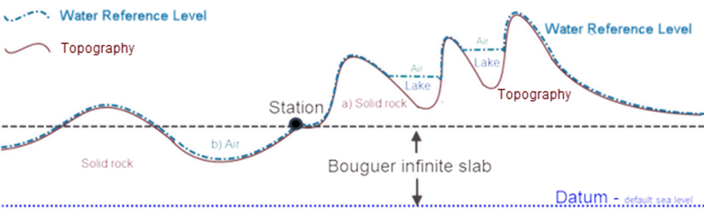
Figure 1: Schematic illustration of Bouguer slab, terrain, and variable water elevations

The magnitude of the terrain effect at each gravity station depends on topography variability, with nearby topography exerting a stronger influence due to the inverse-square law of gravity. Detailed information about nearby topography is necessary, as it significantly affects gravity measurements. Distant features, which exert a weaker gravitational effect, can be represented more generally using larger cell sizes. The Terrain Correction tool decimates the grid as it moves outward from each gravity station for which it calculates the terrain effect.

If you have a detailed local DEM but only a coarse regional DEM, to account for an adequate correction distance, start by invoking Boolean Operations to merge the two grids. Select the grid with the smaller cell size as “Grid 1”, choose the “Or” logic, opt for the maximum grid size, and use the values from Grid 1 in the overlapping area. This resamples the regional grid to the smaller grid increment. The Terrain Correction tool will then automatically decimate this finer DEM as required.

The graph below illustrates the gradual change in the magnitude of the terrain correction as a function of the correction distance for a gravity survey conducted in rugged topography (in red). The topography was scaled to create the other two profiles. The graphs asymptotically approach a limit (thin grey lines) at a distance from the gravity station. Selecting a correction distance at 95% of the asymptote is reasonable. Asymptotes are shown with thin grey lines, the 95% threshold is marked with a dashed line, and the intersection points are indicated by grey bars.

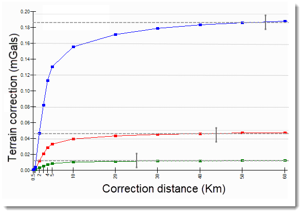
Figure 2: Profiles of terrain correction versus correction distance for three DEM grids of varying reliefs.

The DEM grid used to produce the terrain effect of the red profile has a maximum vertical topographic range of 300 m, with a standard deviation of 67 m. The graph asymptotes near 0.049 mGal, and 95% of this amplitude is reached at a distance of 44 km—an adequate distance for this DEM.

The DEM grid used for the blue profile shows a maximum vertical topographic range of 660 m and a standard deviation of 135 m (approximately double the grid above). The graph asymptotes around 0.196 mGal, reaching 95% of this value at 55 km—again, an adequate distance.

The DEM grid used to produce the terrain effect of the green profile has a maximum vertical topographic range of 165 m and a standard deviation of 32.5 m (half of the first DEM grid). The corresponding graph asymptotes at approximately 0.012 mGal, with 95% of the amplitude reached at 25 km—an adequate distance for this DEM.

Conclusion: There is no one-to-one relationship between a DEM’s vertical relief and the correction distance. You should set the distance to the maximum distance of the available DEM. For very rugged areas, it is generally unnecessary to go beyond 100 km. In relatively flat terrain, much shorter distances yield reasonable results.

Avoid measuring gravity at the edge of sharp relief—such as cliffs or gorges—as terrain correction at these locations will inevitably be less accurate.

In general:

• For relatively flat regions where the variability of the terrain is in the tens of meters, terrain corrections typically range from 0.1 to 1 mGal.

• In hilly regions with variability in the hundreds of meters, terrain effects are on the order of 1 to 10 mGal.

• In mountainous areas, the terrain effect may reach several tens of mGal.

Bathymetric correction follows similar principles; gravity corrections are determined by a combination of the thickness of the water column and the underlying solid material.

Topography Grid

The topography grid is centered on the gravity survey area and should extend at least the correction distance beyond the edges of the survey perimeter. Dummy terrain values are interpolated using a weighted average of the surrounding points.

If the grid does not extend sufficiently beyond the survey area, and the specified correction distance exceeds the gap between the topography grid outline and the survey perimeter, the grid will be extended to meet the required margin. This extension is simply the other edge of the topography grid reflected on the opposite side. However, this is a fallback method and may introduce errors in terrain effect calculations if the nature of the topography changes significantly or if the survey terrain has a regional slope. The correction distance should therefore be selected carefully to avoid introducing errors at stations near the edge of the defined topography grid.

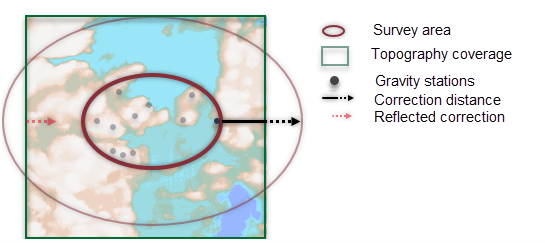
Figure 3: Reflection of terrain elevation on opposite sides

Digital gridded terrain models are often available from government sources and can help simplify the application of regional terrain corrections.

These grids should not be gridded to a cell size significantly smaller than the original sampling accuracy of the DEM data. If the topography grid is produced by gridding the elevation of the gravity survey, the grid cell size should be approximately half the nominal spacing between gravity stations.

Terrain Correction Methods

Terrain corrections are calculated using a combination of the methods described by Nagy (1966)³ and Kane (1962)². The terrain effect is derived using an annular ring segment approximation applied to square prisms. The algorithm sums the effects of four sloping triangular sections that define the surface between the gravity station and the elevation at each diagonal corner. In the intermediate zone, terrain effects are calculated for each point using Nagy's flat-topped square prism method. In the far zone (beyond 16 cells), terrain effects are derived based on Kane's annular ring segment approximation of a square prism.

To calculate the correction at each gravity station, the topography grid is resampled and centered on the station, then extended to the specified correction distance (see Figure 3). The correction is calculated using a series of concentric square zones. The total terrain correction is the sum of the effects from each zone:

• Near zone (Zone 0): A 1-cell radius square ring centered on the station.
• Intermediate zones:
  • Zone 1: Extends from 2 to 8 cells from the station; treated as flat-topped square prisms.
  • Zone 2: Extends from 9 to 16 cells from the station.
• Far zones (Zone 3 and beyond): Concentric flat-topped square rings beyond 16 cells. The number of far zones depends on the defined correction distance.

Each zone is aligned with the next, ensuring consistent spatial coverage. To reduce computation time, the far zones are progressively desampled by a factor of 2, with each cell representing the average of the grid values it covers— see Figure 4, right side:

• Zone 2: Every 4 adjacent DEM cells are averaged into one cell.

• Zone 3: Every 16 adjacent DEM cells are averaged into one cell.

• And so on.

When the Optimize process option is enabled, the desampling factor increases from 2 to 4, further enhancing performance— see Figure 4, left side:

• Zone 2: Every 16 adjacent DEM cells are averaged into one cell.

• Zone 3: Every 64 adjacent DEM cells are averaged into one cell.

• And so on.

Each zone covers the same area but uses coarser resolution as its distance from the station increases. This hierarchical approach ensures that high-resolution detail is preserved where it matters most—near the station—while using lower-resolution data in more distant areas to reduce computational load without significantly impacting accuracy.

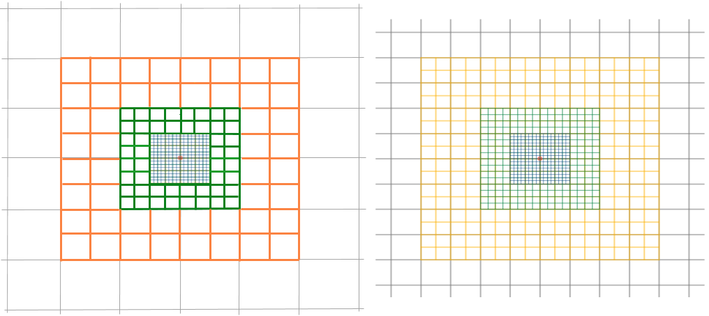
Figure 4: Resampling of DEM for each gravity station by zones

Additional considerations:

• Grid edge reflection: The grid is mirrored at its edges to ensure corrections extend to the required radius.

• Dummy value handling: Any dummy values in the grid are interpolated using adjacent non-dummy values before terrain correction is calculated.

• Outer correction compensation: Beyond the outer (regional) correction distance, the system applies the grid’s average elevation to account for remaining terrain effects.

Equations

Zone 0: Sloped triangle (Kane)

Innermost 4 prisms:

Where:

g = the terrain effect

D = the density

G = the gravitation constant

Zones 1 & 2: Right rectangular prism (Nagy)

1 to 8 cells away from station:

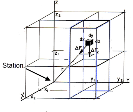
The three bars indicate the limiting values x1, x2 – y1, y2 - z1, z2. The above notation expands to 9 terms, each with a combination of x_i, y_j, z_k.

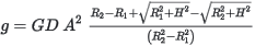
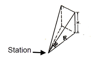
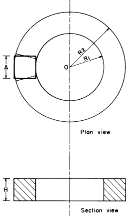
Zone ≥3: Square segment ring (Kane)

Beyond 8 cells away from station up the specified inner distance:

Shipborne and Airborne Surveys

For shipborne and airborne surveys, corrections are calculated as follows: 

• Using the flat-topped square prism approach of [Nagy ,1966]³ for the near and intermediate zones.

• Using the rod formula [Telford et al.,1976]⁴ for the far zone.

Script Mode

The following parameters are available only when executing the current GX from a script:

Terrain correction grid: Contains the correction values beyond the survey area, extended by the specified correction distance. The magnitude of the correction in the terrain correction grid is normalized and scaled to the provided Earth density, then added to the terrain correction calculated from the more finely sampled topography grid. Script Parameter: GRTERAIN.CORGRD

Local slope channel: The local slope of the grid is calculated on the fly; however, if local slopes have been measured at each station, you can specify the slope channel. (The slope is only applicable to Zone 0; see the Application Notes section.) Script Parameter: GRTERAIN.SLOPCH

References

- [1] W. J. Hinze, R.B. Von Frese, A. Saad, Gravity and Magnetic Exploration: Principles, Practices and Applications, (Cambridge University Press, 2013), pp. 134-135.
- [2] M. F. Kane, "A Comprehensive System of Terrain Corrections using a Digital Computer", Geophysics, vol. 27, no. 4 (1962), pp. 455-462.
- [3] D. Nagy, "The Gravitational Attraction of a Right Rectangular Prism", Geophysics, vol. 31, no. 2 (1966), pp. 362–371.
- [4] W. M. Telford, L.P. Geldart, R.E. Sheriff, Applied Geophysics, Second Edition, (Cambridge University Press, 1976), pp. 13-14.
*The GX.NET tools are embedded in the geogxnet.dll file located in the \Geosoft\Desktop Applications\bin folder. To run this GX interactively (outside the menu), first navigate to the bin directory and provide the GX.NET tool in the specified format. See the Run GX topic for more guidance.
Got a question? Visit the Seequent forums or Seequent support
Copyright (c) 2025 Bentley Systems, Incorporated. All rights reserved.
Privacy | Terms of Use