Wiener Optimum (OPTM)

Use the Wiener Optimum option to apply a Wiener optimum filter to your data.

Wiener Optimum Filter dialog options

Inclination	Geomagnetic inclination I, in degrees measured from the horizon.
Declination	Geomagnetic declinationD, in degrees azimuth.
Minimum depth of sources	The depth h (in ground units) at which to interpret the optimum filter from the observed energy spectrum. By default, this depth is taken from the flying height specified in the control file, or from the continuation depth if set by either the Downward Continuation or Apparent Susceptibility options.
Roll-off start (longer) wavelength	The wavelength (in ground units) at which to begin the short-wavelength roll-off (associated with 1/k₀). This parameter must be specified together with the roll‑off end wavelength. By default, k₀ is determined by locating the point where the slope of the observed energy spectrum becomes greater than the slope defined by the depth (1/(4πh)).
Roll-off end (shorter) wavelength	The wavelength (in ground units) at which to end the short-wavelength roll-off (associated with 1/k₁). By default, k₁ = 2 x k₀.
Noise level (log spectral density)	The noise spectral-density estimate θ to be removed by the Wiener filter, expressed as the logarithm of the spectral density (as shown in the second column of the energy spectrum). By default, this noise level is calculated as the average spectral density between k₀ and k₁.

Application Notes

Optimum Wiener Filter

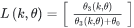
The Wiener optimum filter is designed to remove the effects of white noise from magnetic data. White noise represents high-wavenumber background noise in the spectrum.

Because magnetic signals are strongest in the direction of the inducing geomagnetic field, the signal‑to‑noise ratio varies with both inclination and declination. The optimum Wiener filter accounts for these directional sensitivities during noise reduction, yielding a more accurate reconstruction of the magnetic signal while suppressing high‑frequency noise components.

The filter is defined across three wavenumber ranges:

	for k < k₀
	for k₀ ≤ k ≤ k₁
	for k > k₁

Parameters

I	Geomagnetic inclination, in degrees.
D	Geomagnetic declination, in degrees azimuth.
h	Depth at which the optimum filter is interpreted from the observed energy spectrum. Default: flying height (from the control file) or continuation depth (from Downward Continuation or Apparent Susceptibility), in ground units.
k₀	Wavenumber (cycles/ground unit) where the high‑wavenumber roll‑off begins. Must be specified together with the roll‑off end wavelength. Default: determined by the point where the observed spectrum slope exceeds the slope defined by the depth (1/(4πh)).
k₁	Wavenumber where the high‑wavenumber roll‑off ends. Default: k₁ = 2 x k₀.
φ	Noise spectral‑density estimate to be removed by the filter, given as log spectral density. This is in terms of the log of spectral density as reported in the second column of the energy spectrum. Default: Average spectral density between k₀ and k₁.

Wavenumber Domain Variable Definitions


The following variables are used in the wavenumber domain:
k	Wavenumber increment, used to depict a radially symmetrical variable.	Where: np: number of points cs: cell size
μ	X-component of the wavenumber.
v	Y-component of the wavenumber.
r	Radial component of the wavenumber.
θ	Angular (polar) component of the wavenumber.

Ground unit refers to the survey ground units defined in your grid (e.g., metres or feet). Ground units may be left undefined.

Usage Considerations

The optimum filter is commonly used to remove the theoretical effects of sources lying above a specified depth. Filter parameters can be entered manually or calculated automatically using the energy spectrum.

Although FILTER can calculate filter parameters, you should verify that the interpreted values are reasonable. When the energy spectrum is not smooth, the algorithm may incorrectly choose the starting point for noise estimation—most often selecting a point that is too low—resulting in overly smoothed final maps.

Because the optimum filter can be complex to apply and interpret, a practical alternative is to use a Butterworth filter as a low‑pass filter. Identify the wavenumber corresponding to undesirably shallow sources by interpreting the depth estimate in the energy‑spectrum plot.