MAGMAP Filter Design
Use the interactive filter design dialog to define the Fourier domain filters and to interactively preview the original grid and the filtered grid(s). If the filter file provided in the MAGMAP Filtering dialog is a pre-existing filter control file (*.con), the filter values stored in that file are loaded by default. You can then modify the filter parameters interactively to obtain the best results for your data.
The preview panes allow you to view both the original grid and the resulting filtered grid(s). As you adjust your filter parameters, the results are immediately updated in the Filtered Grid window.
MAGMAP Filtering | Create/Edit Filter dialog options
Spectrum Pane
|
The interactive spectrum graph (see Figure 1) displays the radially averaged power spectrum of the input grid as a function of wavenumber. This spectrum is shown in black. When you define a filter, its radial representation—if one exists—is displayed in blue. The icon  flags filters that do not have a radial representation. The filtered spectrum is shown in red. If multiple filters are applied, each filter and its corresponding output spectrum are displayed in distinct colors. A legend along the bottom of the graph identifies each one. flags filters that do not have a radial representation. The filtered spectrum is shown in red. If multiple filters are applied, each filter and its corresponding output spectrum are displayed in distinct colors. A legend along the bottom of the graph identifies each one.
The range of the abscissa spans from 0 to ½ cell size. For convenience, and because filter parameters are specified in wavelengths rather than wavenumbers, you can toggle the axis display between wavenumber and wavelength (1/wavenumber). This toggle affects only the axis annotation—it does not modify the data in the graph.
To allow finer control over the longer wavelengths (lower wavenumbers), you can increase the minimum wavelength by up to a factor of 10. You can adjust the range by editing the value at the right end of the abscissa.
The ordinate shows the logarithm of the power spectrum on the left and the range of filter coefficients on the right. You can adjust the power spectrum range by editing the upper and lower values of the ordinate..
When you change the graph range, the Reset button  , located at the bottom left of the graph, becomes active. Click this button to restore the initial data range. , located at the bottom left of the graph, becomes active. Click this button to restore the initial data range.
The Spectrum pane is resizable in both directions. To resize the pane, drag the horizontal or vertical resize grip by holding down the left mouse button (seeFigure 2).
|
Filter Definition
This pane is where you define the filter(s) and their parameters. You can choose from a set of 29 available filters, and MAGMAP allows up to four filters to be applied at the same time. Add filters by clicking Add Filter  located at the bottom right of the pane. Each filter has its own set of parameters. The located at the bottom right of the pane. Each filter has its own set of parameters. The  button next to each filter provides a detailed description of that specific filter. button next to each filter provides a detailed description of that specific filter.
After specifying a filter and pressing Enter, all other panes update automatically to reflect the results of the current filter combination. For convenience, low‑pass, high‑pass, and band‑pass filters include live sliders that allow you to interactively preview the effect of their settings.
|
|
Filter #/name
|
Select a filter from the drop-down list. You may define up to four filters.
The following filters are available:
|
|
- Apparent Density Calculation
- Apparent Susceptibility Calculation
- Bandpass
- Butterworth
- Butterworth Bandpass
- Butterworth Notch
- Conversion between Field Components
- Cosine Roll-off
- Cosine Roll-off Bandpass
- Derivative
- Differential Reduction to Magnetic Pole
- Directional Cosine
- Directional Pass/Reject
- Downward Continuation
- Gaussian Regional/Residual
|
- General Radially Symmetric
- Gravity Earth Filter
- High-pass
- Horizontal Integration - X
- Horizontal Integration - Y
- Low-pass
- Notch
- Pseudo-ogravity
- Reduce to Magnetic Equator
- Reduce to Magnetic Pole
- Transform from Magnetic Pole
- Upward Continuation
- Vertical Integration
- Wiener Optimum
|
Fourier domain filters are
commutative, and the order in which the filters are applied does not affect the result.
|
Filter Parameters
|
You will be prompted for additional
parameters depending on the requirements of each filter. Parameters can be adjusted either by moving the available slider controls ( ), or by entering values directly in the parameter fields. After entering a parameter, press Enter to apply the change. The spectra and preview images update automatically. ), or by entering values directly in the parameter fields. After entering a parameter, press Enter to apply the change. The spectra and preview images update automatically.
|
Preview Pane
The preview pane provides an interactive view of both the original grid and the filtered grid(s). The two preview windows are linked, and the cursor location is synchronized between them. The most recently assigned color table for the input grid is used to display both images in the preview pane.
The pane is resizable. To resize it, drag the grip located at the bottom right corner of the pane.
|
|
Original grid
|
This pane displays an image view of your original grid.
If you selected multiple input grids, the Original grid label is replaced with a drop-down list containing all available grids for preview. The first grid in the list is selected by default. From this list, choose the grid you want to preview: 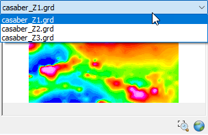
The image in the Filtered grid pane updates automatically to reflect the filter result for the selected input grid.
|
|
Filtered grid
|
This pane displays an interactive image of your filtered grid.
Initially, the pane is empty. Once you define filters, their results appear here. If you have defined multiple filters, the Preview filter result list becomes active, allowing you to view the effects of each filter individually or in combination.
|
|
[Zoom]
|
To zoom into a specific area on both grids, click the Select and zoom to an area of interest button ( ). When you activate this tool, the cursor changes to selection mode in both the Original grid and Filtered grid windows. ). When you activate this tool, the cursor changes to selection mode in both the Original grid and Filtered grid windows.
Use the cursor to draw a box around the area you want to examine, then click inside the box to zoom in.
|
|
[Show entire data extent]
|
Click the Show entire data extent button ( ) to restore the full, unzoomed view. ) to restore the full, unzoomed view.
|
Application Notes
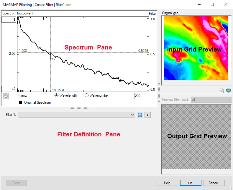
Figure 1: MAGMAP - Interactive filter layout
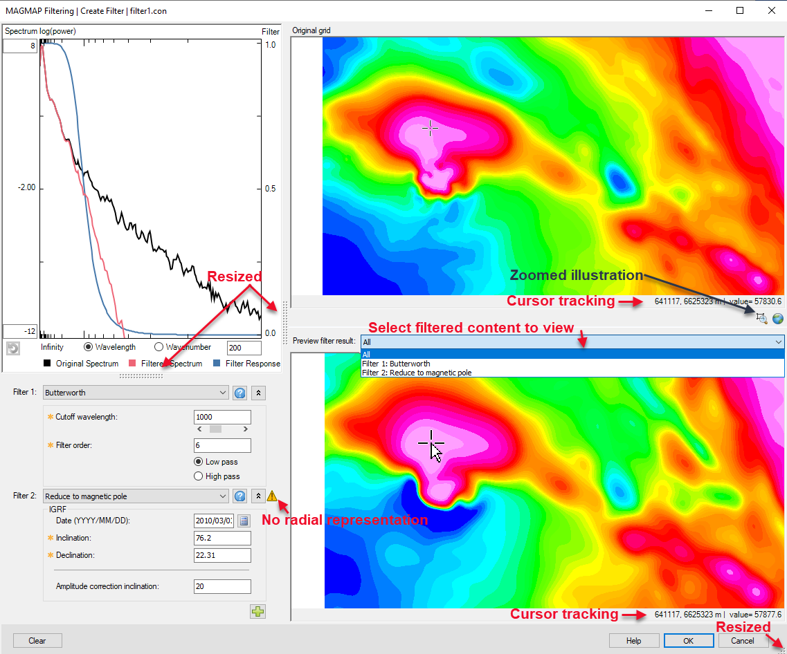
Figure 2: MAGMAP - Interactive definition of filters
Grid Size Consideration
If the input grid is very large, refreshing the graphs and images in the MAGMAP filter window may be slow. To avoid performance delays, when the input grid exceeds 2,048 cells in either dimension, it is automatically decimated to dimensions below 2,048. The decimated grid is saved in the working folder and reused the next time you launch the MAGMAP interactive filter. If you delete the preview grid, MAGMAP will recreate it when needed.
The decimated grid inherits the base name of the input grid with the suffix _preview. Its transform inherits the input grid’s base name with _preview_trn appended. These decimated files are used only for generating the graphs and preview images in the MAGMAP filter window.
The final output grid is always generated from the original, full‑resolution input grid.
Finding Help for a Specific Filter
Once you select a filter, detailed information is available by clicking the button located beside the Filter drop-down or by using one of the links provided below.
To better view the preview panes, Maximize and Minimize buttons are available on the dialog’s title bar. The main Help button is located beside the OK and Cancel buttons at the bottom of the dialog.