
TDEM Waveform and Time Windows
Use the TDEM Waveform and Time Windows tool to specify the time gates to be modelled along with the noise levels for each.
TDEM Waveform and Time Windows dialog options
|
Waveform definition |
The waveform specification can contain either the name of the source database or a comma separated list of defined parameters. |
|
Offset of time windows from start of waveform |
The offset of the designated shutoff time from the beginning of the waveform. The first EM gate containing data may be further offset from the shutoff time.
|
|
[Zoom] |
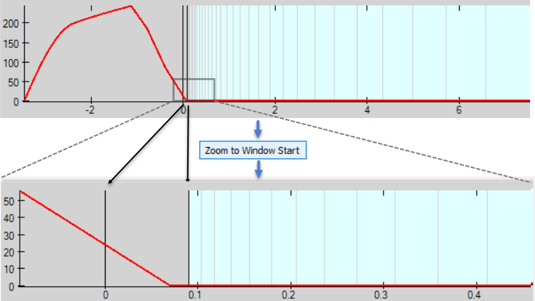
Press the button to enable a 20x zoom toggle that magnifies the time scale around the first receiver time window. Press again the button to go back to full view. |
|
Import Time Windows from File |
The time gates can also be read from a file – see Application Notes below. |
Application Notes
You can easily view and modify your current waveform definition in VOXI Manager:
- In the Data tree, hover the cursor over Windows and Waveform and a tooltip will display your waveform specification if defined.
- Right click Windows and Waveform, then click on Modify:
- If no waveform has been defined yet, the Specify TDEM Waveform dialog will open first in order to define your waveform data for the inversion.
- If the waveform has been defined, TDEM Waveform and Time Windows will open: further modifications to the waveform specification can be made along with time windows selection.
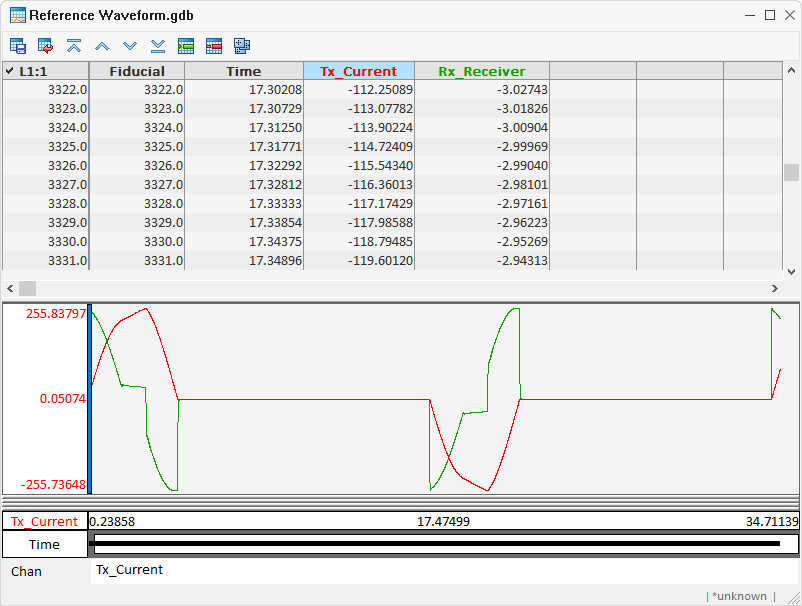
The standard waveform database consists of the fields:
-
Fiducial: Unique fiducial number
-
Time: Time the current was recorded relative to the start of a cycle in milliseconds
-
Tx_Current: Current at transmitter at the designated time in Amps
-
Rx_Receiver: Voltage at receiver, equivalent to dI/dt
This database has as many lines as flights in the project. The waveforms may vary somewhat from flight to flight. This tool averages them and sends half of the averaged waveform to the inversion engine.
The time gates of the EM decay array are generally supplied in a separate file and should be loaded onto the EM decay channel prior to invoking VOXI. The zero time of the time gates start at the designated shutoff time. The fields of the decay sampling are:
-
Start: Start time of the gate
-
End: End time of the gate
-
Middle: Middle time of the gate
-
Width: Width of the gate
VTEM Decay Sampling scheme Window Start End Middle Width
Milliseconds Noise Floor (pV/Am4)
4 0.018 0.023 0.021 0.005 0.0792 5 0.023 0.029 0.026 0.005 0.064 6 0.029 0.034 0.031 0.005 0.046 7 0.034 0.039 0.036 0.005 0.034 8 0.039 0.045 0.042 0.006 0.026 9 0.045 0.051 0.048 0.007 0.0208 10 0.051 0.059 0.055 0.008 0.0156 11 0.059 0.068 0.063 0.009 0.014 12 0.068 0.078 0.073 0.010 0.01216 13 0.078 0.090 0.083 0.012 0.01052 14 0.090 0.103 0.096 0.013 0.00864 15 0.103 0.118 0.110 0.015 0.00712 16 0.118 0.136 0.126 0.018 0.0056 17 0.136 0.156 0.145 0.020 0.0044 18 0.156 0.179 0.167 0.023 0.0036 19 0.179 0.206 0.192 0.027 0.0028 20 0.206 0.236 0.220 0.030 0.0022 21 0.236 0.271 0.253 0.035 0.002 22 0.271 0.312 0.290 0.040 0.0016 23 0.312 0.358 0.333 0.046 0.00132 24 0.358 0.411 0.383 0.053 0.0011 25 0.411 0.472 0.440 0.061 0.00096 26 0.472 0.543 0.505 0.070 0.00084 27 0.543 0.623 0.580 0.081 0.00073 28 0.623 0.716 0.667 0.093 0.00065 29 0.716 0.823 0.766 0.107 0.00059 30 0.823 0.945 0.880 0.122 0.00056 31 0.945 1.086 1.010 0.141 0.00053 32 1.086 1.247 1.161 0.161 0.00049 33 1.247 1.432 1.333 0.185 0.00046 34 1.432 1.646 1.531 0.214 0.00042 35 1.646 1.891 1.760 0.245 0.0004 36 1.891 2.172 2.021 0.281 0.00038 37 2.172 2.495 2.323 0.323 0.00036 38 2.495 2.865 2.667 0.370 0.00034 39 2.865 3.292 3.063 0.427 0.00032 40 3.292 3.781 3.521 0.490 0.00031 41 3.781 4.341 4.042 0.560 0.0003 42 4.341 4.987 4.641 0.646 0.00029 43 4.987 5.729 5.333 0.742 0.00027 44 5.729 6.581 6.125 0.852 0.00026 45 6.581 7.560 7.036 0.979 0.00024 46 7.560 8.685 8.083 1.125 0.00023 47 8.685 9.977 9.286 1.292 0.00022 48 9.977 11.458 10.667 1.482 0.00021 49 11.458 13.161 12.250 1.703 0.00021
The above two tables are shown on the graph of the waveform dialog (see illustration below). In the illustration, the shutoff time is set at 3.4506 ms. The EM decay array start time 0.018 ms is relative to the shutoff. Thus, it occurs at the absolute time 3.4186 ms. Furthermore, the first few gates are normally not used.
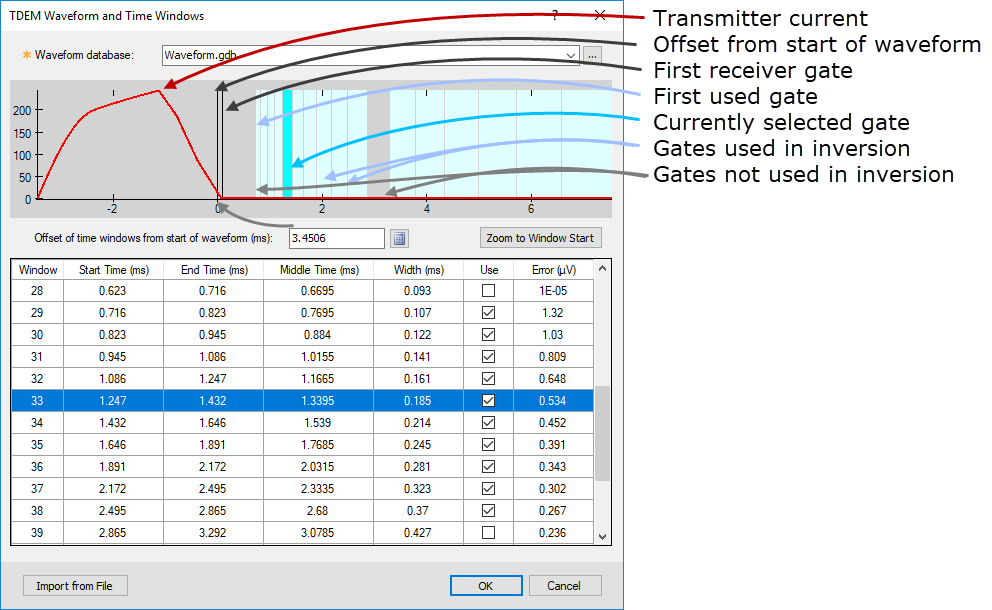
Prior to the inversion, you can further manipulate the settings, for example you could determine which gates are passed to the inversion by checking on/off the Use boxes in the dialog. You can also manually edit the error values.
In the above table, the first 6 fields are always present, but the next fields are subject to the fit error chosen. They are described below for each Fit error selection:
Fit error -> Fraction of standard deviation
-
Std..Deviation: the standard deviation of each gate is calculated and displayed
-
Fraction: a numeric value <1.0 that the St. deviation is multiplied by to produce the error for that gate
-
Minimum value: The error for each gate is set to either this threshold value or St. Deviation x Fraction, whichever is larger.
Fit error -> read from channel: if the standard deviation of the EM array is pre-calculated and loaded on the EM array channel, simply use it.
-
Multiplier: prior to inversion, the preloaded values for each gate can be scaled by this multiplier to generate the error values.
Fit error -> Relative error
-
Relative error fraction: For each observation, the error for each gate is set to a fraction of that gate’s value
-
Minimum value: The error for each gate of each observation is set to either this threshold value or the calculated relative error, whichever is larger.
Fit error -> Error channel: No additional fields, the errors are read from the specified array channel.
The Zoom button allows you to zoom in to the start of the Receiver time.
Got a question? Visit the Seequent forums or Seequent support
© 2024 Seequent, The Bentley Subsurface Company
Privacy | Terms of Use