Structural Trends

When modelling and calculating interpolants structural trends can be applied when there is a gradual shift in the direction of the continuity that precludes the use of a global trend, perhaps due to flows.

A structural trend localises trend modelling to indicate changes in direction of continuity. A variety of inputs can be used to inform a structural trend: structural data disks or lineations, a mesh surface, or triaxial trend ellipsoids imported from Driver. The resulting structural trend is a continuous function that can determine, for any given point of interest, the trend orientation and magnitude specific and appropriate to that location.

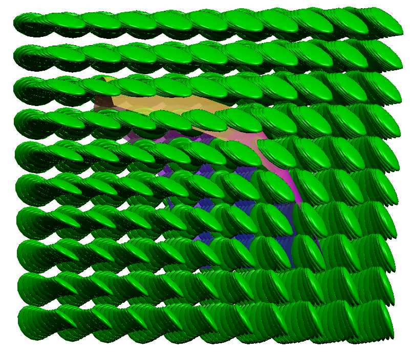
When displayed in the scene, the structural trend is rendered as a grid of oblate ellipsoids. The orientation of the disk gives the direction of the anisotropy. The size of a disk is proportional to the anisotropy strength.

The above scene depicts the result when the structural trend is a Non-decaying type. Because the strength of the trend does not decay, all the ellipsoid disks are the same size but may point in different directions.

You can also select a structural trend type with an effect that decays toward a general background trend:

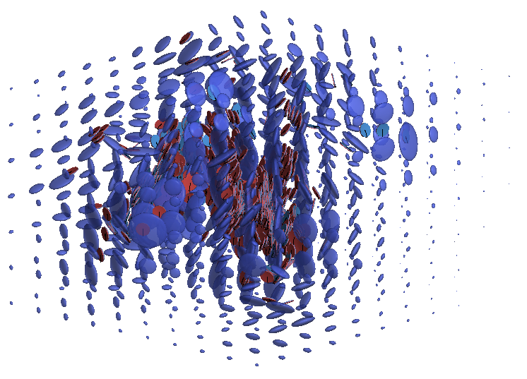
Where there are no ellipsoids or very small ellipsoids, the trend is isotropic.

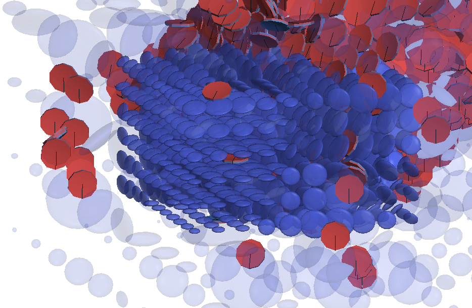
Structural trend ellipsoids are a discrete visualisation of the continuous structural trend function, depicting the strength and direction of the anisotropy at specific defined locations. The visualisation grid can be changed to visualise the function in space at the desired granularity or resolution. In this example, a smaller extents region was also specified to limit the high resolution spacing to a specific area:

Clustering Settings and Visualisation

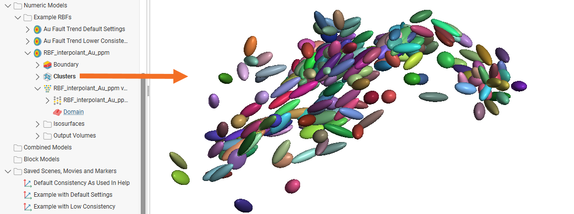
Clusters represent the local anisotropy of a grouping of input data. Each cluster can be represented in the scene as a trend ellipsoid.

Clusters take data points that are in close proximity with similar local anisotropy and infer a representative local anisotropy. This is done by defining Clustering Settings to break the points down into a grid representing the Minimum cluster size then, based on the Anisotropic consistency threshold, the algorithm merges neighbouring mini-clusters with a similar anisotropy. The mini-clusters are merged until the Maximum cluster size is reached or until the anisotropy of the neighbouring mini-clusters are too inconsistent to merge.

Clusters appear in the project tree when a structural trend is applied. Clustering requires the use of a Spheroidal interpolant. It is not supported when using Linear interpolants.

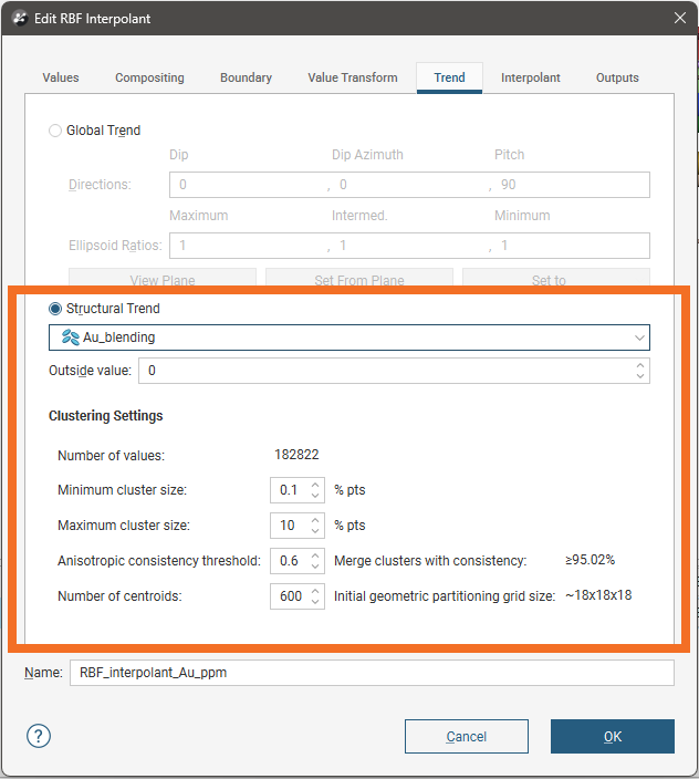
Double-click a Clusters object in the project tree to open the edit window. When a structural trend is selected that uses Strongest along inputs, Blending, and Non-decaying, the tab will appear as follows:

Where Triaxial blending structural trends are selected, the Number of centroids and Initial geometric partitioning grid size fields will not appear.

You can select a Structural Trend from the list of available trends.

The Outside value sets the expected background value for the region. The outside value is factored into the interpolation algorithm and lowers the interpolated value in the areas away from the known data points. To increase the projection area outside of the area with data, the outside value can be increased to a value just below the cut-off value.

The Clustering Settings are provided for adjustment of the structural trend algorithm behaviour. These are some of the settings that can be adjusted:

Minimum cluster size and Maximum cluster size constrain how the interpolation algorithm infers clusters when applying the structural trend. They are specified as a percentage of the total number of input data points available. During structural trend clustering, the data points are clustered into small regions down as far as the minimum cluster size. These mini-clusters are then merged into larger clusters if the mini-clusters are sufficiently consistent in their respective anisotropies, up to the maximum cluster size. It cannot define clusters containing fewer data points than the minimum cluster size, and the cluster cannot have data points exceeding the maximum cluster size.

The Anisotropic consistency threshold controls how similar clusters need to be to be in order to be merged into a larger cluster.

Number of centroids specifies how many centroids are in a three-dimensional geometric partitioning grid. The approximate number of centroids along each axis of the resulting grid is described by the Initial geometric partitioning grid size shown in the window. This initial geometric partitioning grid is created in the interpolation process while clustering the data. The data inputs are broken down into the initial geometric partitioning grid’s cellular units as a primitive step, from which the clusters are then constructed, merged and simplified. This initial geometric partitioning grid cannot be viewed in the scene.

Increasing the number of centroids will result in a more stable model output when more input data is added to the interpolant using the structural trend, especially if that data causes the extents to change. However, more centroids will also mean that it is more likely that isolated regions might be harder to link to other regions, despite an obvious trend implying that the regions are probably connected. This can be aggravated by a large Minimum cluster size that forces the initial mini-clusters to enclose all the points in a grid cell, which could also result in adjacent mini-clusters being sufficiently inconsistent in anisotropy that they cannot link up into consolidated clusters.

Reducing the number of centroids and the resolution of the initial geometric partitioning grid may contribute to being able to model these as connected regions. However, reducing the number too much could result in significant impacts on parts of the model distant from a region where new data is added.

If your model is producing many small and isolated interpolated surfaces, that you expect should be consolidating due to an obvious trend, you might try one or a combination of the following:

Increasing the Maximum cluster size
Decreasing the Consistency threshold

This may produce a result closer to what you expect. Similarly, if a model is producing large and consolidated interpolated surfaces, that you expect could be described better using multiple smaller regions, one or a combination of the following could drive the algorithm to infer this expectation:

Decreasing Maximum cluster size
Increasing the Consistency threshold

Changing the Minimum cluster size may also contribute in both cases, but a direct relationship cannot be stated. The larger the minimum cluster size, the less the local structural inputs will have influence. Increasing the minimum cluster size will combine more points into initial mini-clusters, and this may contribute to consolidating surfaces, but if the minimum cluster size is too high and the Number of centroids is too high, a counter-productive effect can result in inconsistent clusters that cannot be merged.

As a guiding rule of thumb, using a minimum cluster size of 0.1% the number of points, and a maximum cluster size of 10% the number of points will often produce good results.

To illustrate, compare the effects of two different sets of parameters:

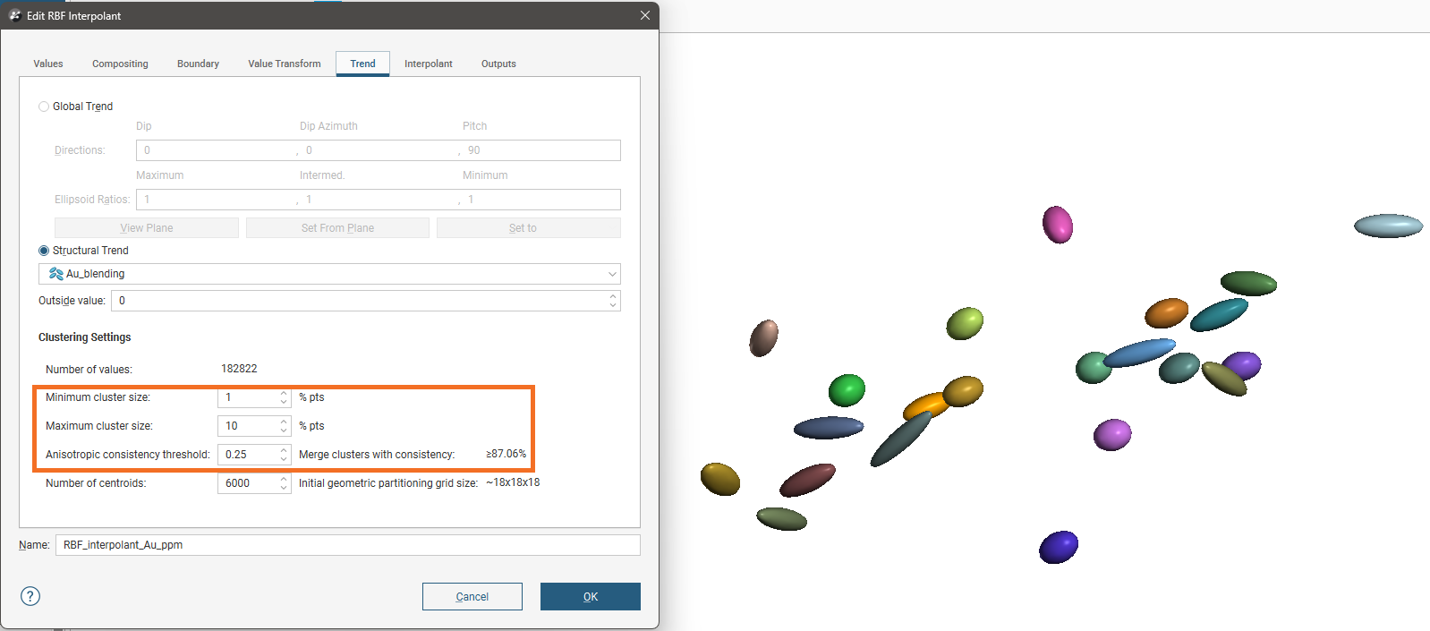
In the first example, the clustering settings used are:

Minimum cluster size: 1% pts
Maximum cluster size: 10% pts
Anisotropic consistency threshold: 0.25.

This produces a smaller number of clusters that are larger and more consolidated.

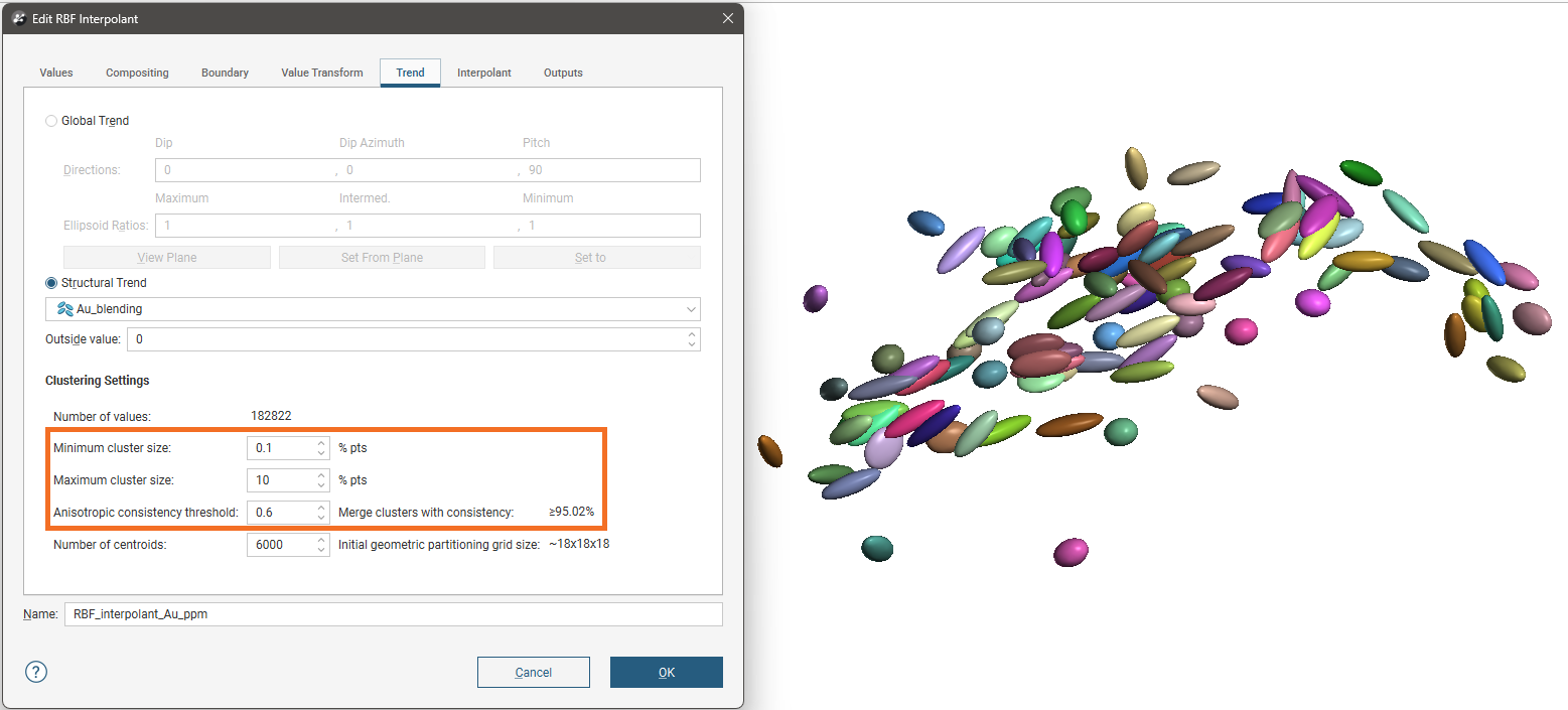
In the second example, the clustering settings used are:

Minimum cluster size: 0.1% pts
Maximum cluster size: 10% pts
Anisotropic consistency threshold: 0.6

This produces a larger number of clusters that are smaller with each representing few data points.

As you adjust these clustering parameters, use caution and watch for patterns or artefacts that the adjustments provoke in the isosurfaces produced by interpolants. You may also need to adjust the strength of the anisotropy to achieve a geologically sensible result. This is done in the Inputs tab of the structural trend itself, found in the Structural Modelling folder in the project tree. See Creating a Structural Trend for more information on how to do this.

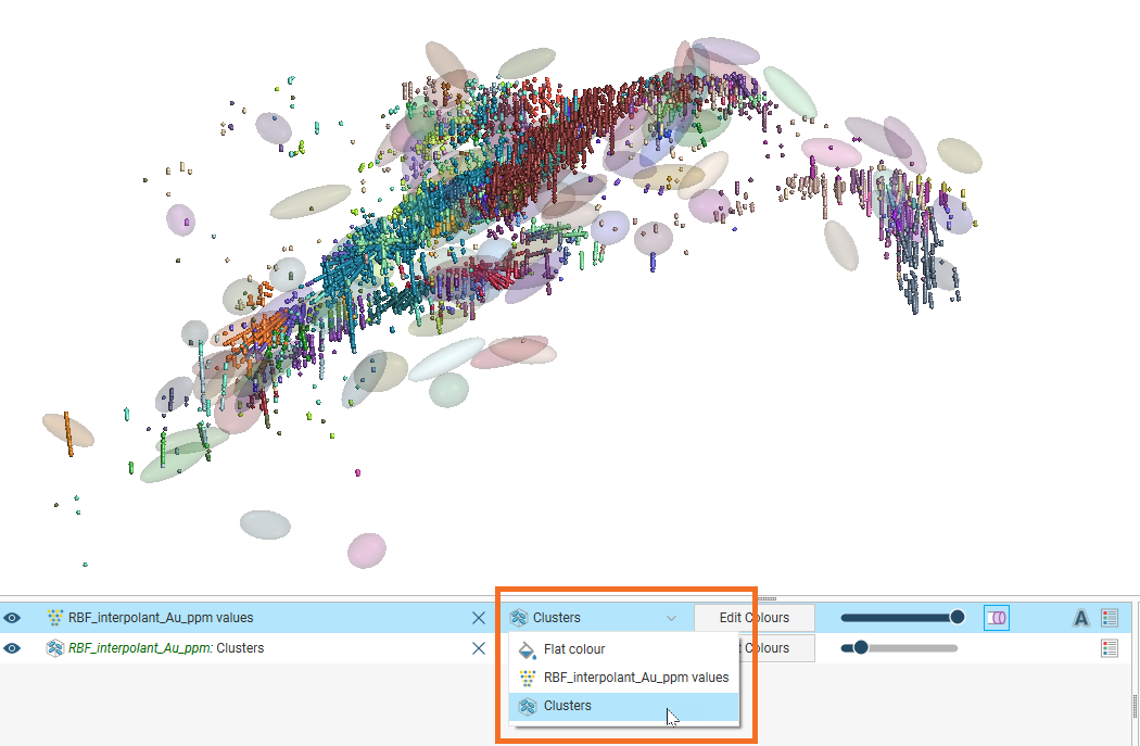
Visualising the ellipsoids in the scene can give an indication of the local anisotropy applied as an input to the model.

To see the points in each cluster, add the points into the scene setting the colouring in the shape list to Clusters. The points will be coloured to match the ellipsoids representing the local anisotropy of the points in the cluster. This can be useful in determining how you might adjust the clustering parameters.