Block Models
You can create the following types of block models in Leapfrog Energy:
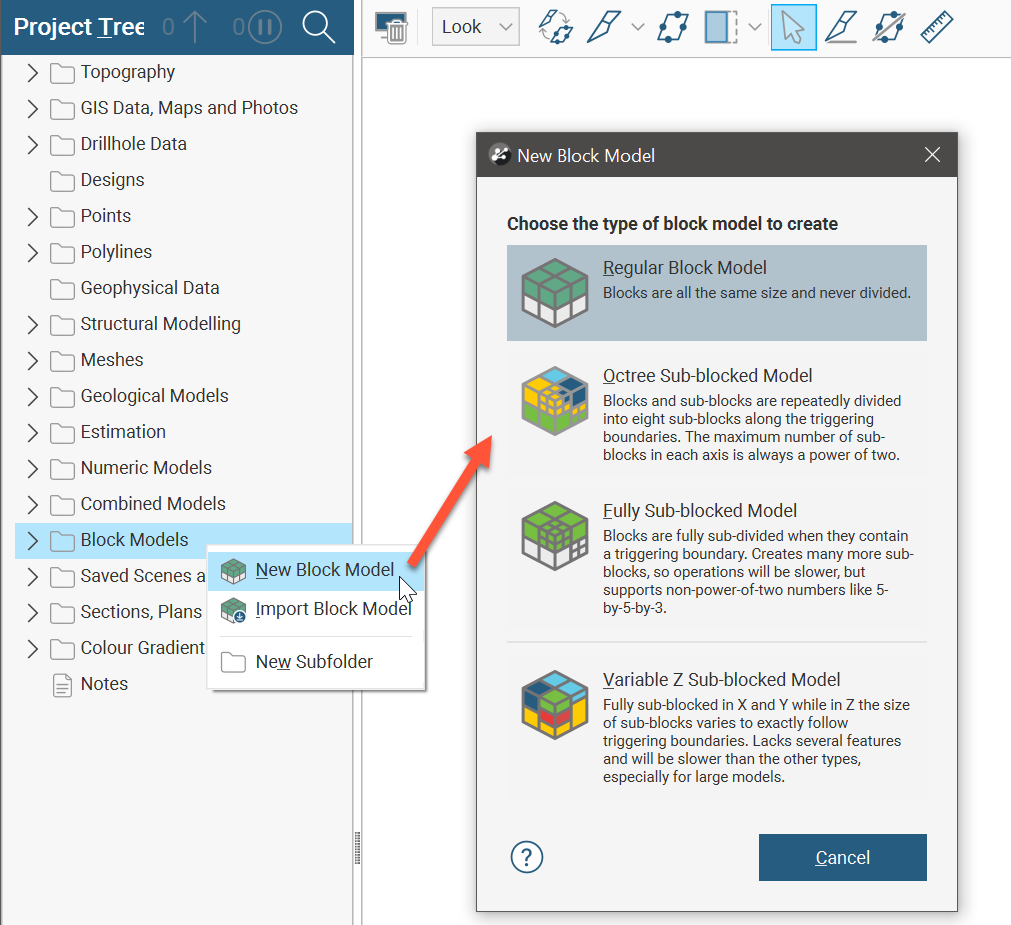
- Regular block models. A regular block model has blocks that are all the same size and are never divided.
- Octree sub-blocked models. An octree sub-blocked model has blocks that are repeatedly divided into eight sub-blocks where selected triggering surfaces intersect the blocks. Instead of dividing a block entirely into small sub-blocks when sub-blocking is triggered, the block is first divided in half in a particular direction, and then only the partitioned blocks that still trigger a further division are divided into smaller units. This creates a series of sub-blocks of different sizes, and because many are larger than the smallest sub-block and the smallest sub-blocks only exist where a contact requires it, processing can be more efficient.
- Fully sub-blocked models. With fully sub-blocked models, blocks are fully sub-divided when they contain a triggering boundary. This can create many sub-blocks and so processing a fully sub-blocked model can be slower than processing an octree sub-blocked model. In contrast to octree sub-blocked models, however, fully sub-blocked models support block subdivisions using numbers other than power-of-two numbers. Fully sub-blocked models do not support variable height sub-blocks.
- Variable Z sub-blocked models. Variable Z sub-blocked models are fully sub-blocked in X and Y, but in Z the size of the sub-blocks varies to exactly follow triggering boundaries.
You can also:
- Regularise octree sub-blocked models, fully sub-blocked models and variable-z sub-blocked models into a block model that is not sub-blocked. Regular block models can be regularised into a block model with larger block dimensions and fewer blocks. See the Regularising Block Models topic.
- Export block models. See the Exporting Block Models topic.
- Import block models in different formats. See the Importing Block Models topic.
The rest of this topic describes:
Creating New Block Models
To create a new block model, right-click on the Block Models folder and select New Block Model. In the window that appears, select the type of block model you wish to create:
For more information on each block model type, see the following separate topics:
- Creating a Regular Block Model
- Creating a New Octree Sub-blocked Model
- Creating a Fully Sub-blocked Model
- Creating a Variable Z Sub-Blocked Model
Block Model Volume Filters
Mesh volumes can be assigned to block models as volume filters. Right-click on a block model in the project tree and select New Volume Filter. Select the volume from the list of available objects.
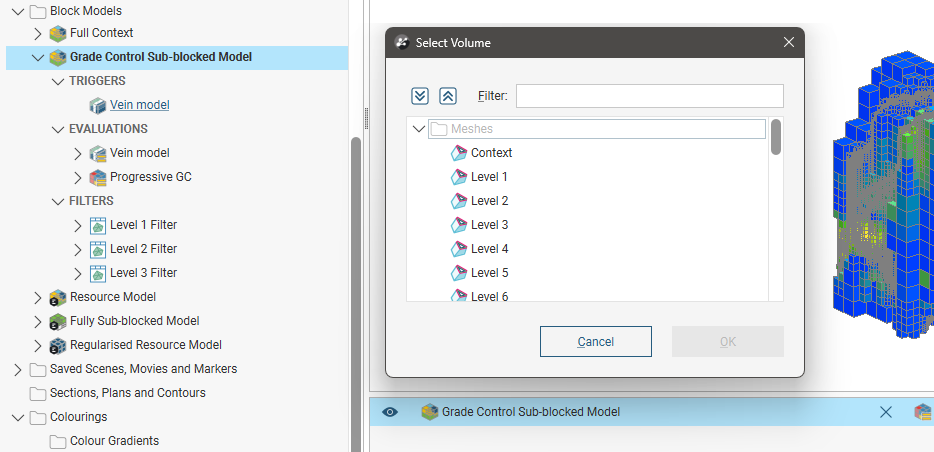
Volume filters will appear as selectable options in the shape list properties panel’s Query filter, where the volume filter can be selected to show only the parts of the block model within the selected volume.
Displaying a Block Model
Along with the standard Slice mode options in the shape list properties panel for making sliced views of the block model, there is a 2D slice mode option. This option displays a regular block model, an octree sub-blocked block model, or a fully sub-blocked model at the surface of the slicer.
2D slice is not available for variable-z sub-blocked models.
The 2D slice has several advantages over viewing a thick slice, where entire blocks may be missing or may be hidden by foreground blocks well in front of the slicer, depending on your slice thickness. Here, the display of a standard thick slice suggests there are holes in the block model, whereas in reality the centroids of those ‘missing’ blocks are outside of the thick slice and so not displayed:
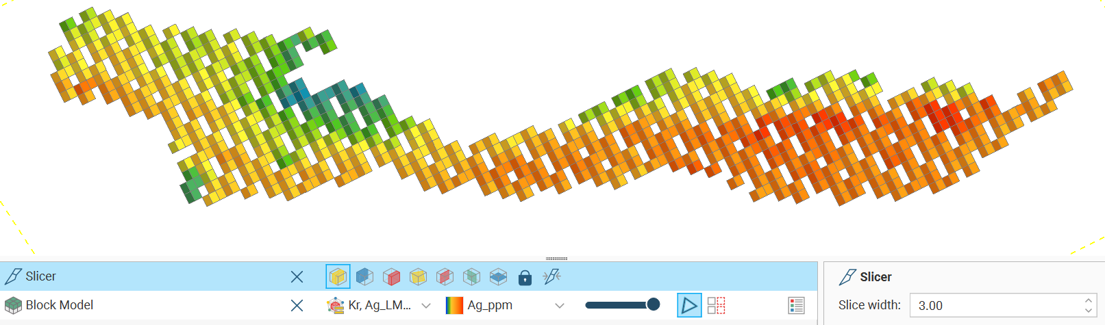
When 2D slice mode is enabled, each block intersecting the slicer is depicted:
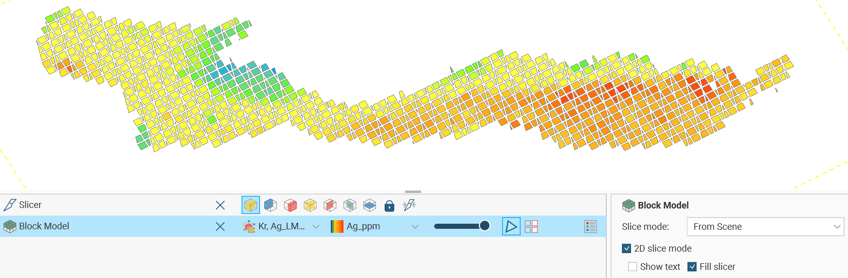
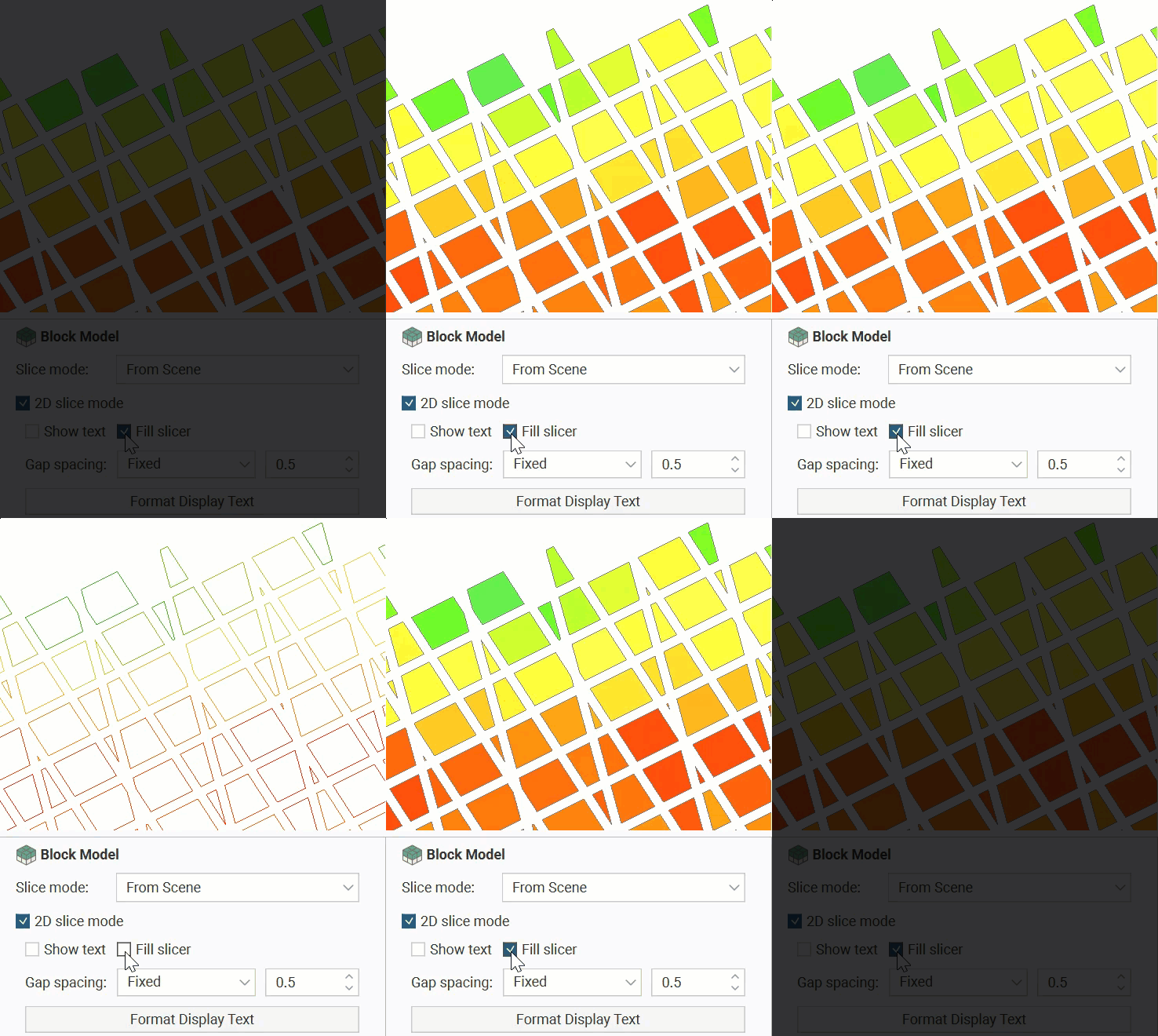
The Fill slicer option provides the choice between an outlined shape for the intersection of each block with the slicer, or a filled shape.
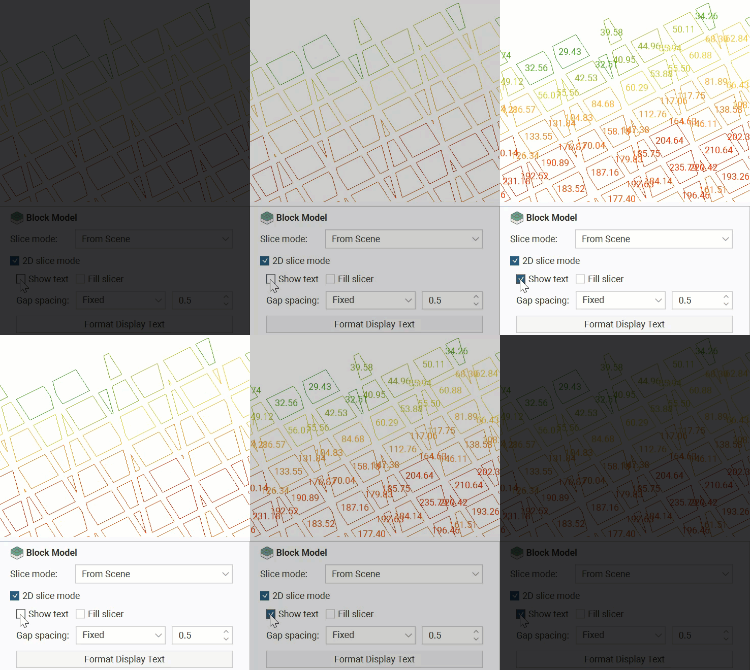
The Show text option provides the choice between seeing a value on screen for each block intersecting the slicer, or not. The default value is the value for the column selected to colour the block model.
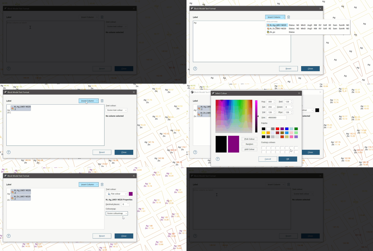
Click the Format Display Text button to open the text format dialog in which you can customise the scene text displayed for each block, including the column values displayed and the colouring of different parts of the text label.
See Formatting Text Displayed in the 3D Scene for more information on how to use the text formatting dialog.
The size of the gap around a block can also be customised. With regular block models, octree sub-blocked models and fully sub-blocked models, you can specify a fixed gap size to be used between all blocks. With regular block models you can alternatively choose a data column and the gap around each block will be proportional to the selected value of that column for the block. The selected value can also be the result of a calculation. These variable gaps are created by scaling each block with a scaling factor between 0 and 1, linearly mapped from 0 to the selected attribute maximum.
 Choosing between an outlined shape or a filled shape
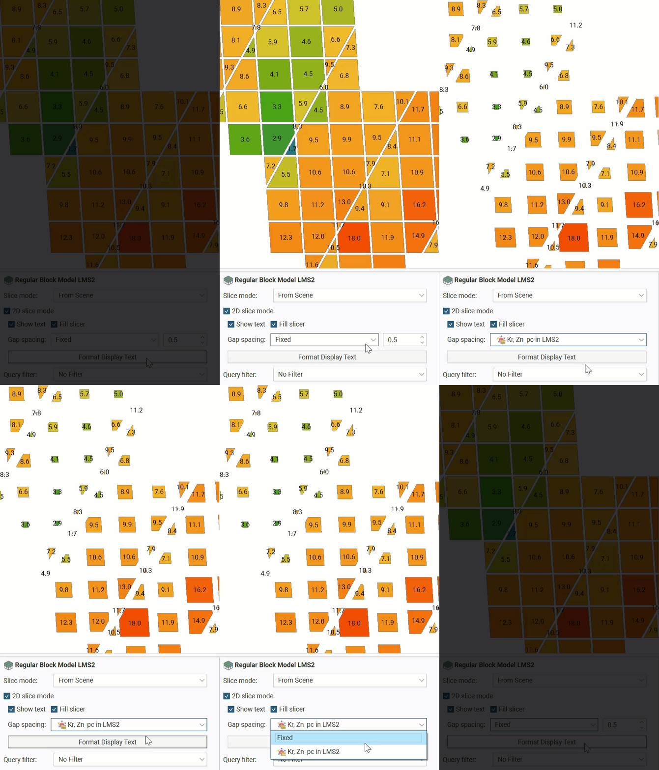
Block models can also be added to a section layout, where they will have an appearance similar to the 2D slice mode view. This presentation option includes a query filter and an index filter. See the Section Layout Editor topic for more information on designing section layouts.
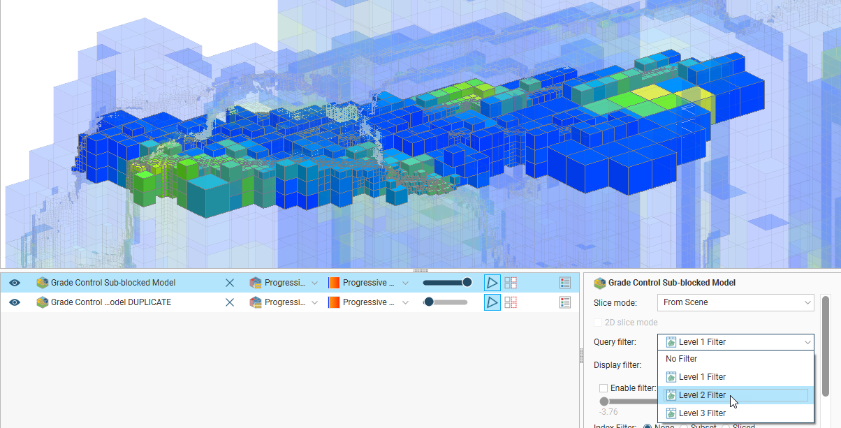
When a block model is displayed in the scene, there is a Query Filter option that includes filters created in Calculations and Filters.
The Query filters list will also contain volume filters. To set a volume filter on a block model, see Block Model Volume Filters.
The Display filter provides a further option for selecting relevant portions of the model to display in the scene view. The default option is From Scene, which applies the selected column found in the shape list. Other evaluations can be selected from the list to create a filter independent of the column shown in the shape list. Enable filter will apply the filter when ticked.
- If a category column is chosen, a Select Categories button can be used to select the discrete categories to show.
- If a value column is chosen, a value range filter is shown.
- If a date column is chosen, a date range filter is shown.
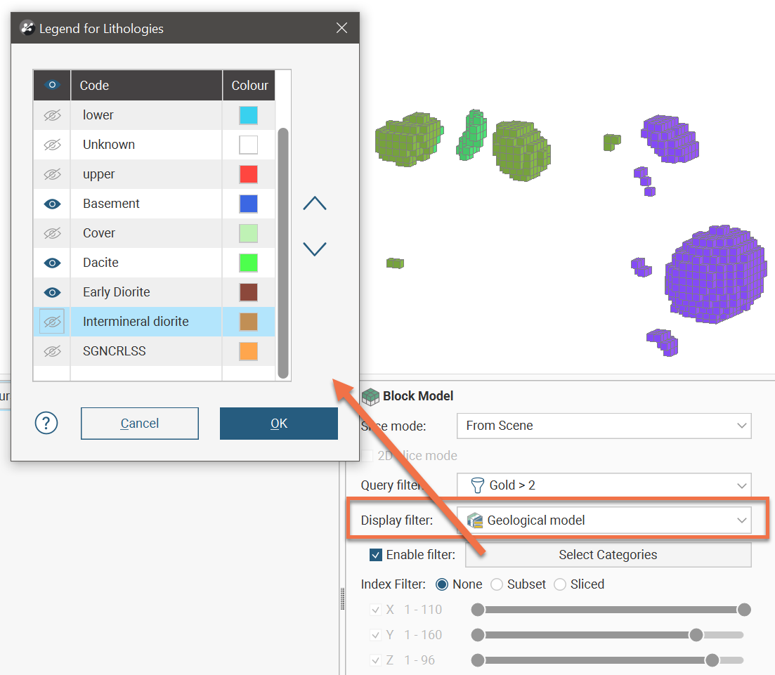
For more information on how to use the Display filter, see the Using the Display Filter section in the Filtering Data in the 3D Scene topic.
When a block model is displayed in the scene, there is an Index Filter option for displaying the grid:
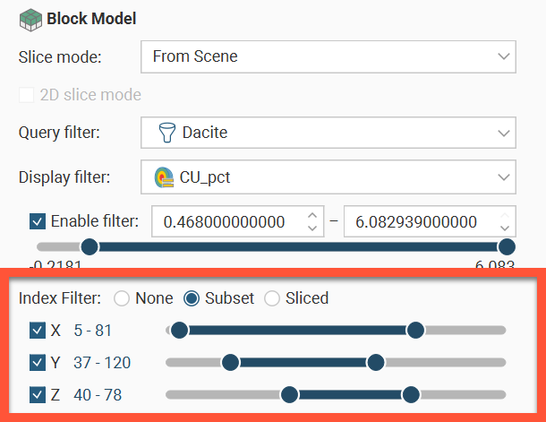
The Index Filter can be set to None, Subset or Sliced.
- Subset shows the union of the selected X, Y and Z ranges.
- Sliced shows the intersection of the selected X, Y and Z ranges.
The X, Y and Z ranges each use a range slider.
Range sliders have two modes: coarse control and fine control. Here a range slider is used for a set of values that ranges from 1 to 160; it is displayed in dark blue, to show the full range of values in coarse control mode:

You can restrict the data displayed by dragging on the handles. Here the range of values is restricted to 1 to 50:

You can click and drag on the selected range to change the values displayed:

To switch to fine control, double-click anywhere along the range slider. Here the range of 52-101 has been expanded along the whole slider, giving you more control over the position of the range end points:
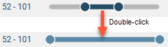
The slider is displayed in light blue in fine control mode.
Now you can use the handles to further restrict the range displayed:
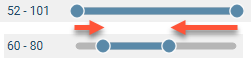
Right-click on the slider to return to coarse control and the full range of values. Here, right-clicking reverts to coarse control, with the range restricted to the original range of 52-101:
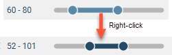
Viewing Block Model Statistics
To view statistics on a block model, right-click on the model in the project tree and select Statistics. The following options are available:
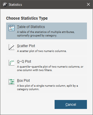
The Table of Statistics option is described in more detail below. See the Saved Statistics topic for more information on the other options.
Right-clicking on a block model evaluation or a numeric calculation and selecting Statistics opens a univariate graph for the selection. See the Univariate Graphs topic for more information.
Table of Statistics
You can view statistics for all evaluations and calculations made on a block model broken down into categories and organised by numeric evaluations and calculations. To view statistics, right-click on a block model in the project tree, select Statistics then select the Table of Statistics option.
You can view statistics for as many numeric and category columns as you wish. When you have at least one Category column selected, you can organise the information displayed in two ways: Group by Category or Group by Numeric. Here, statistics are displayed organised by the category data columns:
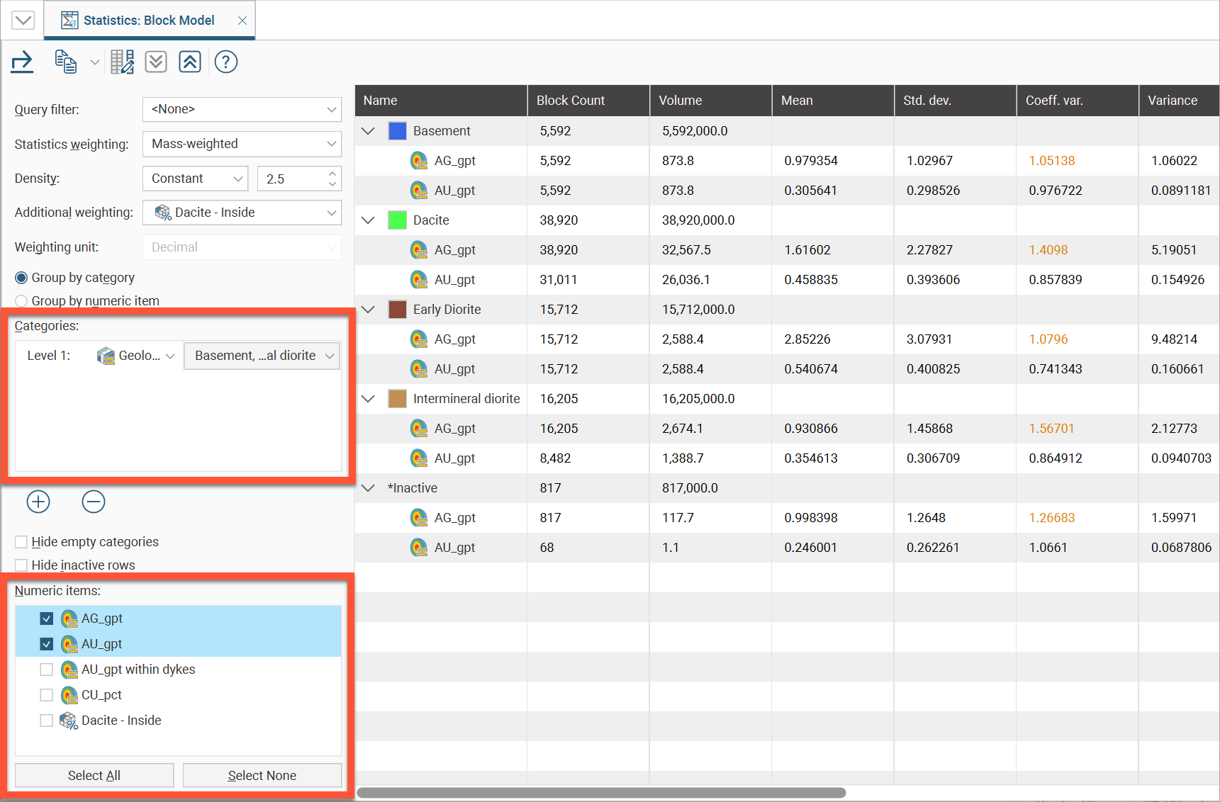
The Query filter option uses a related filter to constrain the dataset to a selected subset.
Statistics can be Un-weighted, Volume-weighted or Mass-weighted. Select the option you require from the Statistics weighting list.
When using mass-weighting, you can also set the Density to be a Constant value that you specify, or you can use one of the columns in the table.
You can select an Additional weighting from the available table columns in the dropdown list. You may need to specify the Weighting unit as Decimal or Percentage if the column selected is not a proportion column. This Additional weighting column is especially useful to use with a proportion column so that only the proportion of a block containing the desired grade is included in the report.
The Categories list provides category classification options. When selected, the set of statistics measures for each evaluation or numeric calculation will be shown for each category.
You can hide empty categories (those with a count of zero) and inactive rows using the options below the Categories list:
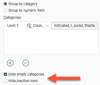
Group by category and Group by numeric column provide options for the table organisation. You can also change what columns are displayed in the table by clicking the Edit columns button ( ). This opens a window in which you can select the columns that are displayed in the table:
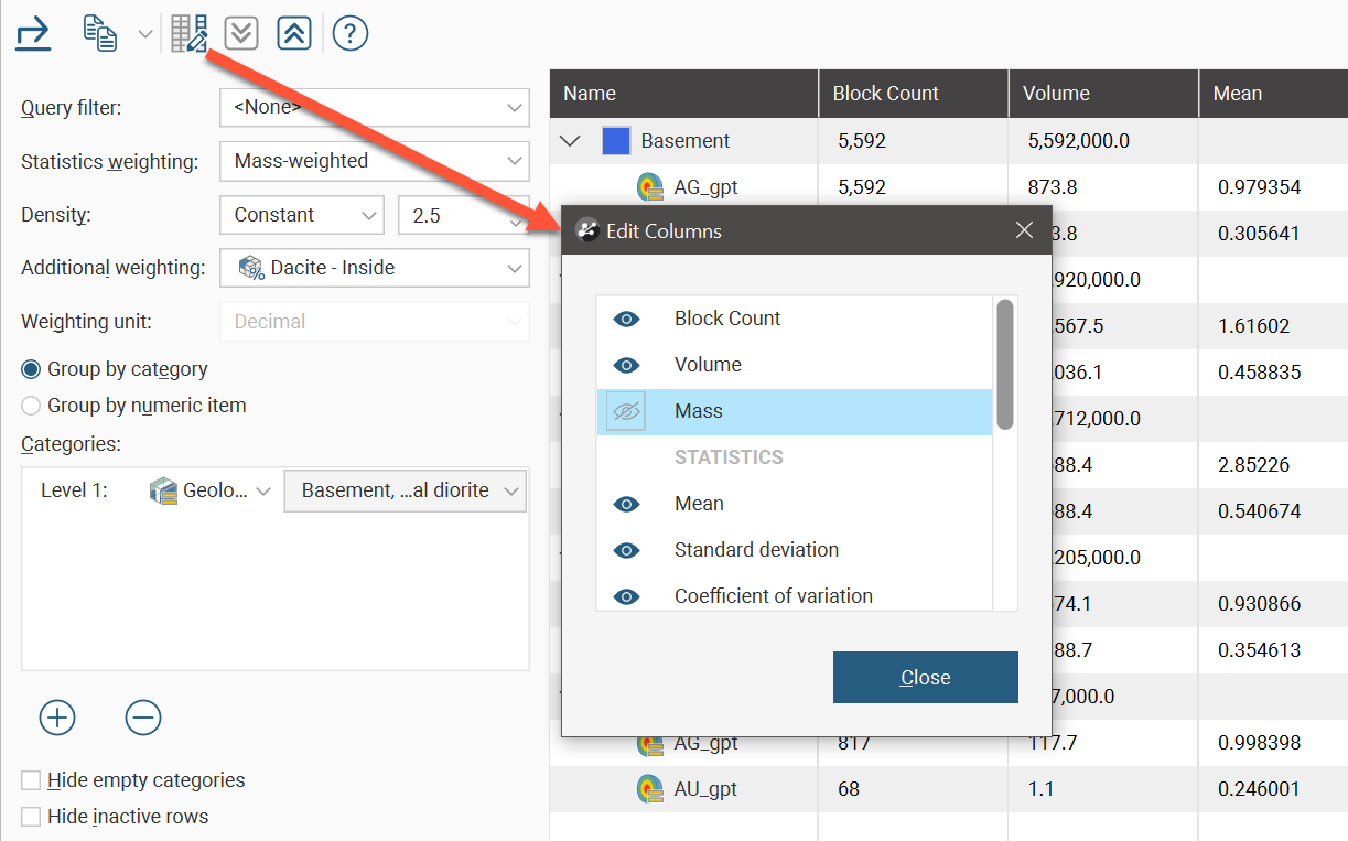
Click rows to select them, and select multiple rows by holding down the Shift or Ctrl key while clicking rows. You can then copy rows by clicking the Copy button ( ), which allows you to copy the selected row(s) or all rows in the table.
The arrow buttons quickly expand ( ) or collapse (
 ) rows.
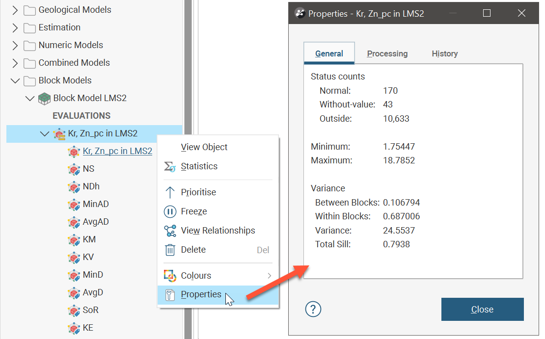
The block model evaluation object has its own Properties window with useful statistics. One important section is the Variance section, providing the variance Between Blocks and Within Blocks, useful for calculations applying Krige’s Relationship and determining the variance correction factor and block dispersion variance.