Back-Flagging Drilling Data

Evaluating geological models on wells creates a new lithology table containing the lithologies from the selected model. This is useful for validating models created from drilling data as you can generate statistics for the correlation between modelled geology and drilling data.

To created a back-flagged drilling data table, right-click on a drilling dataset in the project tree and select New Evaluation Table. The New Evaluation Table window will appear:

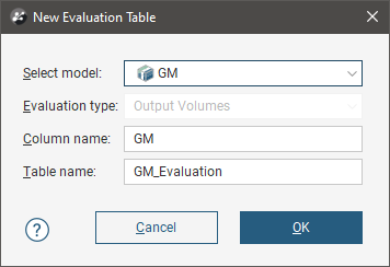
Select the model to use and enter names for the column and table.

When the selected model is a faulted model, the Evaluation Type setting determines whether the model’s output volumes, faulted output volumes or fault blocks are evaluated.

Click OK to create the new table, which will appear in the project tree as part of the drilling dataset. The new table contains From, To and Lithology columns defined using the intersection between the model’s output volumes and the wells.

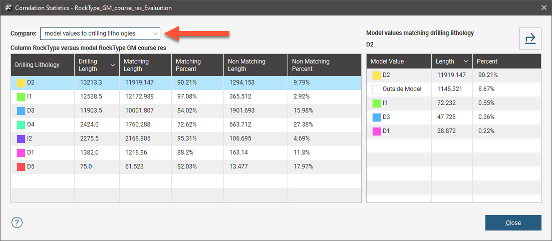
For output volume evaluations, you can view the correlation between modelled geology and actual logged well segments. To do this, right-click on the table and select Statistics. In the Correlation Statistics window, you can compare model values to drilled lithologies or vice versa.

See:

• Comparing Modelled Values to Drilling Lithologies
• Comparing Drilling Lithologies to Modelled Values
• Refining the Geological Model to Improve Correlation Statistics
• Creating a Merged Table Including Assay and Geological Model Lithologies

Comparing Modelled Values to Drilling Lithologies

Comparing model values to drilling lithologies shows how accurately drilling lithologies are modelled in the selected geological model. High matching percentages for drilling lithologies in the left-hand side of the window mean the model closely matches the drilling data for that lithology:

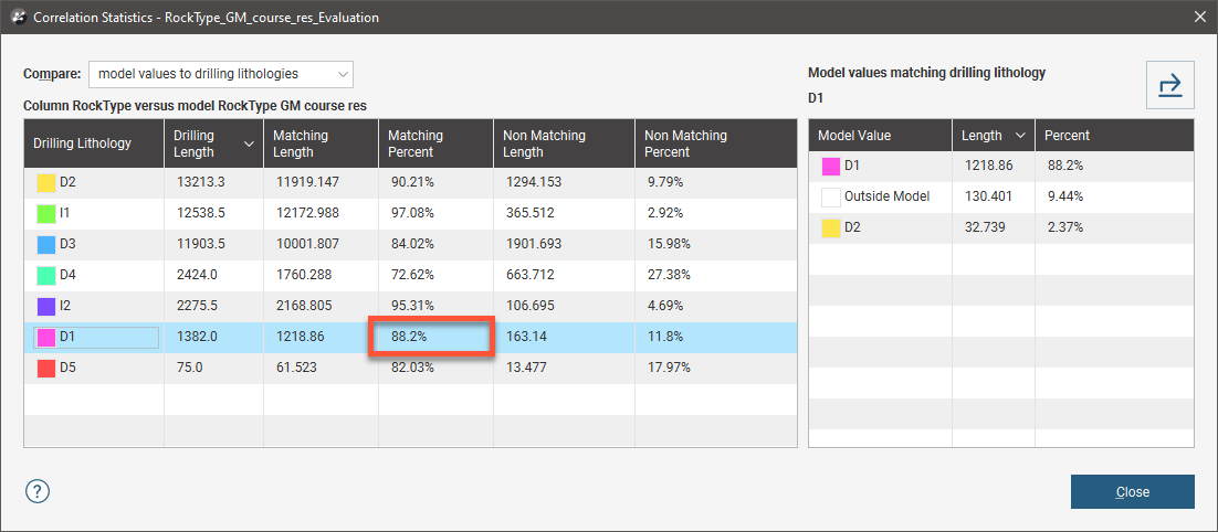
The right-hand side of the window shows the composition of the modelled values for the selected Drilling Lithology. Here, D1 in the geological model corresponds to D1 in the lithology data for 88.2% of the length of the well. D1 in the model is actually D2 for 2.37% of the length of the wells, and 9.44% of the drilled D1 values fall outside of the boundary of the geological model.

In the images that follow, we will look at the correlation between the D5 drilling lithology and modelled D5. Here, two drilling data tables are displayed with the D5-D4 contact surface from the geological model:

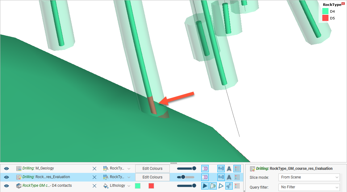
The inner wells show the original drilling data. The outer wells show the geological model back-flagged onto the drilling data table. In the highlighted well, we can see there is a discrepancy between the actual lithology data and that modelled. When we view correlation statistics for this model, we can see that this discrepancy is explained by the fact that 17.97% of the D5 drilling length is modelled as D4:

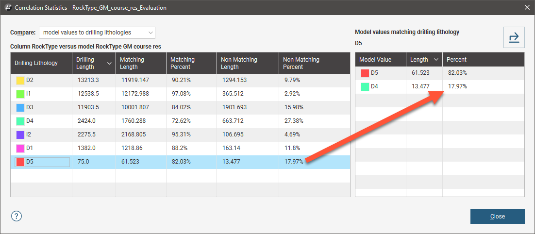
You might consider this an acceptable match, but if it is too low, there are several ways to refine the geological model so that the geological model more closely reflects the original wells, which are discussed below. For this example, we will adjust the resolution of the geological model. The modelled segment now corresponds more closely to the original drilling data:

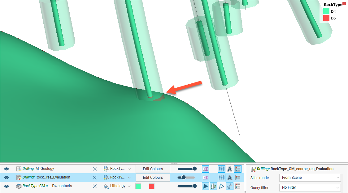
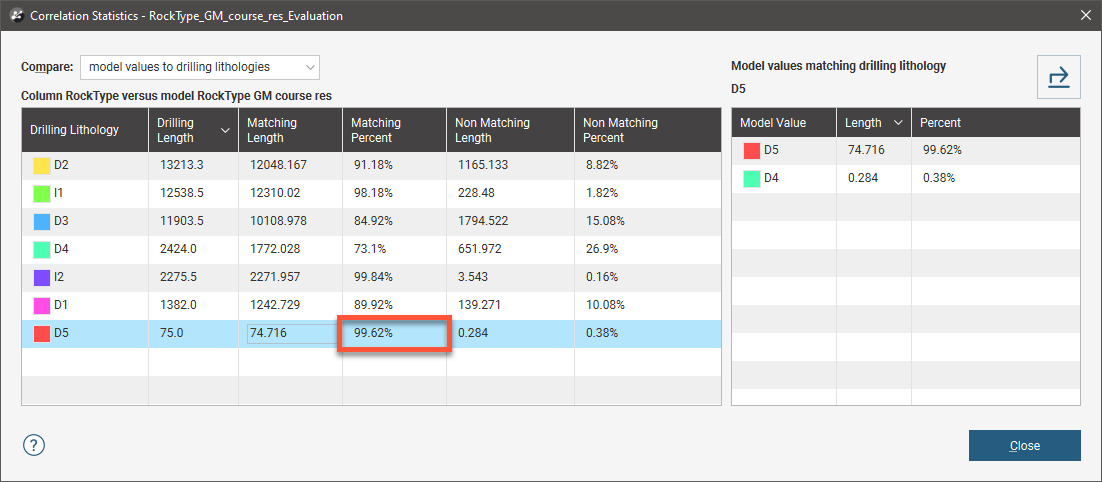
Viewing the correlation statistics shows that 99.62% of modelled wells now match the original data:

Comparing Drilling Lithologies to Modelled Values

Comparing drilling lithologies to model values shows the lithological composition of modelled values. Again, high matching percentages in the left-hand side of the window mean the model closely matches the drilling data for that modelled lithology:

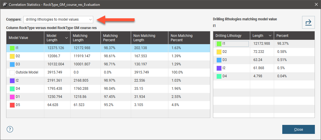
The non-matching percentage indicates how much of the modelled lithology is not the drilling lithology. You can see in the right-hand side of the window the lithologies that make up the non-matching portions of the modelled value.

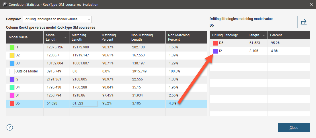
In the images that follow, we will look at the correlation between the D5 drilling lithology and modelled D5 once again. The non-matching percentage is 4.8, and on the right-hand side of the window, we can see that this is exclusively drilling lithology I2:

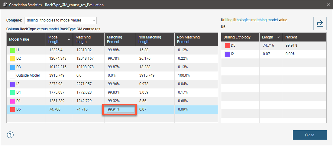
Adjusting the resolution of the geological model improves the matching percentage to the point where only 0.09 percent of the D5 modelled value is drilling lithology I2:

Refining the Geological Model to Improve Correlation Statistics

If the matching percentages are too low for the lithologies of interest, there are several ways to refine the geological model so that the geological model more closely matches the wells:

• Reduce the resolution of the geological model or of its contact surfaces. See Surface Resolution for a Geological Model and Surface Resolution in Leapfrog Energy.
• Add more data to the model’s surfaces. See Adding Data to Surfaces.
• Snap surfaces to the data used to create them. See Honouring Surface Contacts.

Creating a Merged Table Including Assay and Geological Model Lithologies

Creating a back-flagged evaluation table will result in a new table like this:

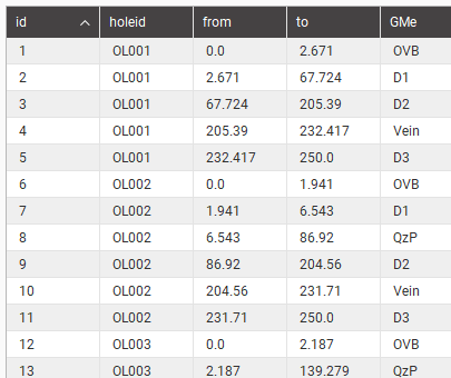
To obtain a table that includes both assay and back-flagged geological model lithologies, create a merged table as described in Merging Drilling Data Tables. The result will be a merged table like this:

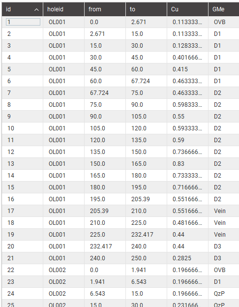
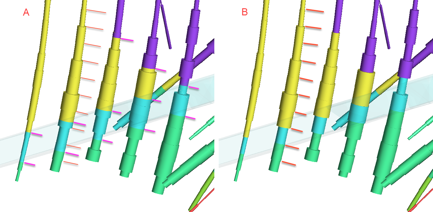
Note that this merged table will split assay intervals where the geological model showed a transition from one lithology to another, as shown above at lines 1 and 2 , and also lines 6 and 7, and so on. Below, in scene A, a modelled vein cutting across wells is illustrated. The drillhole diameter is indicating the assay value and the colour is indicating the lithology. Thin orange lines have been over-draw to show the original assay intervals, while the thicker pink lines show new intervals created by the merging of the tables. An alternative that utilises the existing interval midpoints when allocating the geological modelling lithology as an additional column is illustrated in scene B. If this strategy is preferred, see Evaluated Column From Geological Model.