
Anisotropy grids and global anisotropies
Anisotropy grids and global anisotropies are regularisation techniques. Driver provides two strategies to re-evaluate, or regularise, local ellipsoids:
- Creating an anisotropy grid re-evaluates the local ellipsoids as a regularly spaced grid of ellipsoids.
- Creating a global anisotropy re-evaluates the local ellipsoids as a global ellipsoid, approximating the average trend in the data.
This topic describes those strategies, along with how to publish or export the results. It is divided into:
- Creating an anisotropy grid
- Creating a global anisotropy
- Publishing and exporting anisotropy grids and global anisotropies
Creating an anisotropy grid
An anisotropy grid renders the anisotropies on a grid of locations as opposed to on the drilling locations. It can be used to capture local changes in continuity across the entire data area. It can also evaluate anisotropy away from the data values.
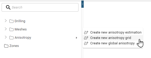
To create an anisotropy grid, right-click the Anisotropy folder in the project tree and select Create new anisotropy grid.
The New Anisotropy Grid window will appear:
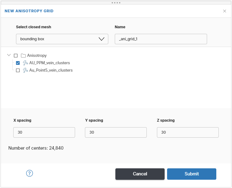
Options are:
- Select closed mesh. Select the mesh as a domain to create the anisotropy grid within.
- Select an anisotropy. Select the top level Anisotropy folder to select all or individually select an anisotropy.
- Name. Each anisotropy grid will be labelled using the attribute’s name appended with the Name entered here. In this example, the complete name of the anisotropy grid would be AU_PPM_ani_grid_1.
- Grid Spacing. Enter the required spacing between the output grid nodes. Driver will adjust to the limits of your data areas and allow for a maximum of 100,000 centres. Choose the largest possible length scale that still captures the scale of anisotropic change in the dataset. The grid spacing does not need to be the same for all grids in the project.
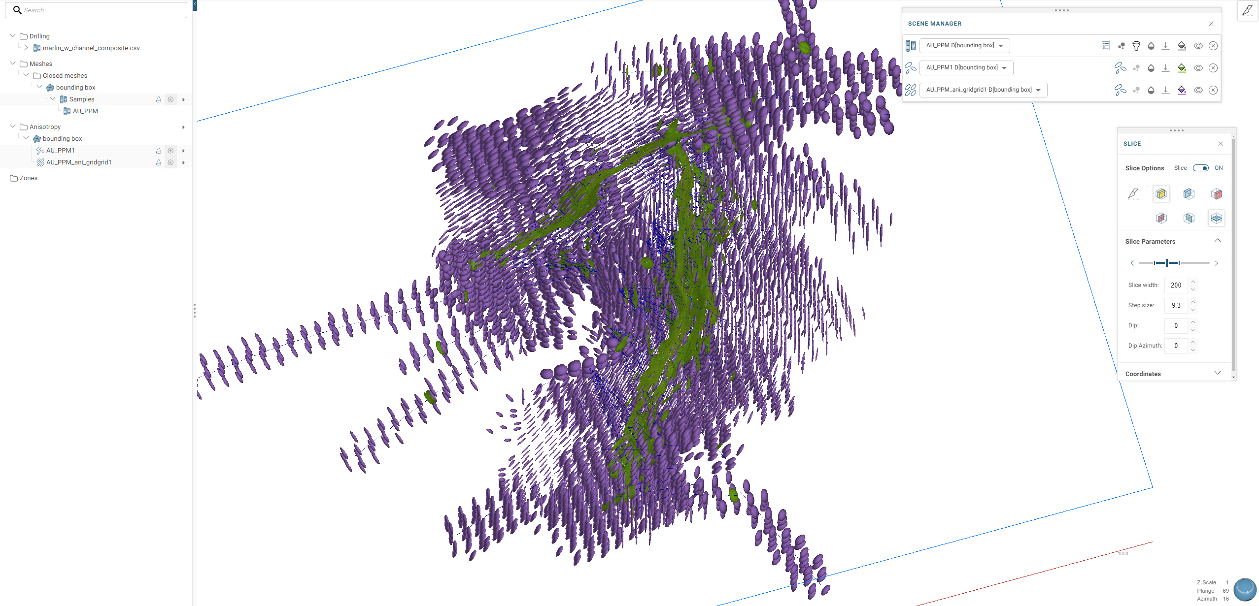
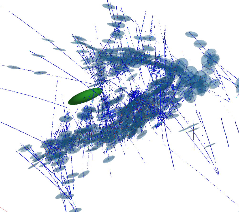
The anisotropy grid is saved to the Anisotropy folder. It is a field of ellipsoids that can be viewed in the scene alongside other objects. For example, here an anisotropy estimation is displayed as green ellipsoids converted to a regular grid:
Creating a global anisotropy
For many modelling uses, the presence of locally-varying anisotropic continuity may be unnecessary as the deposit clearly demonstrates a simple continuity without the presence of complex locally-changing trends. In these scenarios, the unstructured anisotropy estimation objects can be simplified into a global anisotropy that averages all contributing ellipsoids into a single ellipsoid.
To create a global anisotropy from an anisotropy estimation, right-click on the Anisotropy folder in the project tree and select Create new global anisotropy.
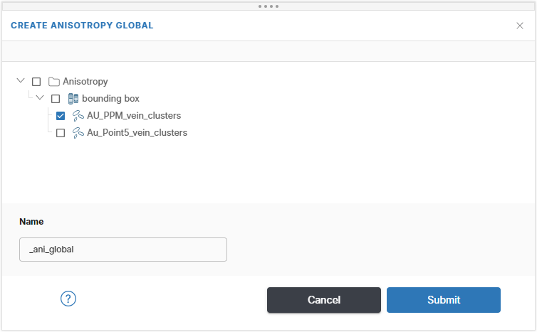
In the New Global Anisotropy window, select the anisotropy estimation to create the global anisotropy from, here AU_PPM_vein_clusters is selected. Also provide a name suffix. Each will automatically be labelled using the attribute's name appended with the name entered here. In this example, the complete name would be AU_PPM_ani_global.
The new global anisotropy will be created as a single ellipsoid that can be viewed in the scene in a similar manner to anisotropy estimations. The ellipsoid will be positioned at the centre of the data inside each domain.
Publishing and exporting anisotropy grids and global anisotropies
Anisotropy grids and global anisotropies in a Driver project can be published to Seequent Evo or downloaded to your local hard drive.
When publishing to Evo, there are three choices:
- Planar structural data. This publishes only the principal ellipsoid plane as structural discs.
- Lineations. This publishes only the major axis direction as a lineation.
- Ellipsoids. This publishes all ellipsoid data as a local ellipsoid geoscience object.
Published objects will appear in the project workspace’s Geoscience objects tab.
The only option for exporting anisotropy grids and global anisotropies to a local file is as ellipsoids in *.csv format. The *.csv file contains the ellipsoid configurations (using the Leapfrog rotation convention), ellipsoid sizes and additional metadata. A *.zip file will be downloaded that contains the ellipsoid file.