Structural Data
In Leapfrog Geo, you can create and edit planar structural data tables directly or from other objects in the project. Structural data can also be used to create and edit many surfaces. Downhole planar structural data and lineations can also be imported, although structural data imported in this way cannot be edited.
This topic describes how to work with structural data in Leapfrog Geo. It covers:
- Creating New Planar Structural Data Tables
- Importing Planar Structural Data
- Importing Lineations
- Displaying Structural Data
- Viewing Statistics on Structural Data
- Assigning Structural Data to Categories
- Editing the Orientation of Planar Structural Data
- Declustering Planar Structural Data
- Setting Elevation for Structural Data
- Estimating Planar Structural Data
See Stereonets and Form Interpolants for information on tools for analysing structural data.
Leapfrog Geo calculates strike using the American right-hand rule; when looking in the strike direction, the plane should dip to the right.
Creating New Planar Structural Data Tables
There are two ways to create a new planar structural data table in Leapfrog Geo:
- Create a new table as part of creating or editing another object. See Editing Surfaces With Structural Data.
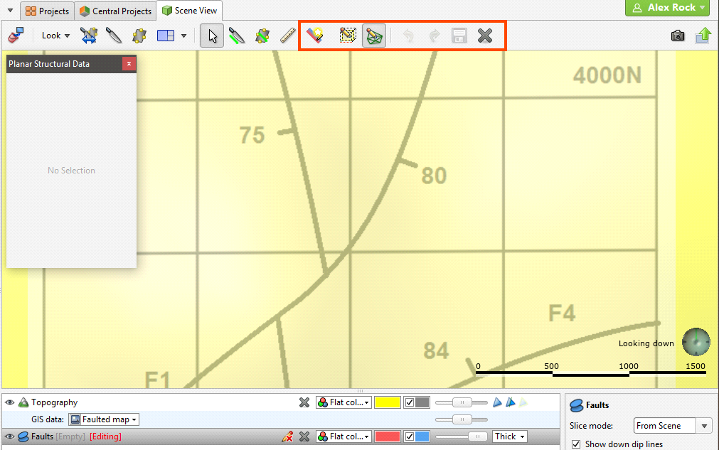
- Create a new table using the Structural Modelling folder. Use this technique when, for example, you are creating structural data points from a map or image. Right-click on the Structural Modelling folder and select New Planar Structural Data. In the window that appears, enter a name for the new table and click OK.
Before creating the new data table, add the map, image or data object you wish to work from to the scene and orient the scene for drawing the new data points.
When a new structural data table is created, it will be added to the scene. The Planar Structural Data window will open, together with a set of tools for adding structural data points:
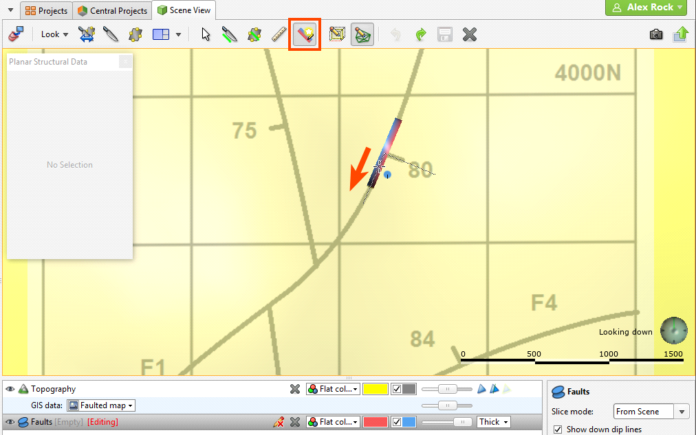
Click on the New Structural Data Point button (![]() ) and click and drag along the strike line in the scene to add a new data point:
) and click and drag along the strike line in the scene to add a new data point:
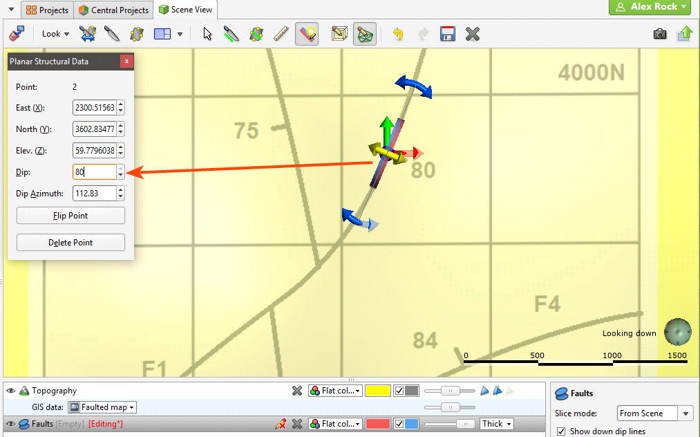
You can adjust the data point using the controls in the Planar Structural Data window:
Importing Planar Structural Data
Leapfrog Geo supports planar structural measurements in .csv or text formats. This topic describes importing structural data tables that include location information. Downhole structural data can also be imported, as described in Importing Downhole Structural Data.
Structural data containing location information can be imported from:
- Files stored on your computer or a network location. Right-click on the Structural Modelling folder and select Import Planar Structural Data. You will be prompted to select a file.
- From any database that runs an ODBC interface. Right-click on the Structural Modelling folder and select Import Planar Structural Data via ODBC. See Selecting the ODBC Data Source below.
For each of these options, once the data source is selected, the process of importing the data is the same. Leapfrog Geo will display the data and you can select which columns to import:
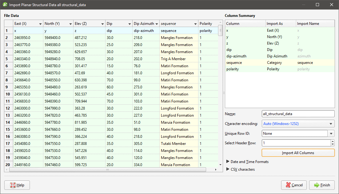
Leapfrog Geo expects East (X), North (Y), Elev (Z), Dip and Dip Azimuth columns. The Polarity column is optional. The Base Category column can be used for filtering data once it has been imported.
Click Finish to import the data. The structural measurements will appear in the Structural Modelling folder.
Once the data has been imported, you can add new columns and rows and reload the data, which is described in the Working With Data Tables topic.
Selecting the ODBC Data Source
When importing planar structural data from an ODBC database, you will need to specify the ODBC data source. Enter the information supplied by your database administrator and click OK.
Once the data source is selected, the import process is similar to that described above.
Importing Lineations
Lineations containing location information can be imported from files stored on your computer or a network location in .csv or text formats. To do this, right-click on the Structural Modelling folder and select Import Lineations. You will be prompted to select a file.
Leapfrog Geo expects East (X), North (Y), Elev (Z), Trend and Plunge columns. The Polarity column is optional. The Category column can be used for filtering data once it has been imported.
Click Finish to import the data. The lineations will appear in the Structural Modelling folder.
Once the data has been imported, you can add new columns and rows and reload the data, which is described in Adding and Updating Data for Existing Tables in the Working With Data Tables topic.
Displaying Structural Data
Planar structural data is displayed as disks and lineations are displayed as cones. There are several ways to change how this data is displayed. In the scene below, planar structural data is displayed using the Flat colour option, with positive (red) and negative (blue) sides shown:
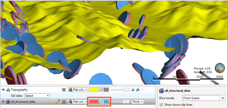
You can change the colours used to display the positive and negative sides using the controls in the shape list. You can also display the data points as Thick disks, Flat disks or as Outlined flat disks. You can change the Disk radius and the Disk size using the controls in the shape properties panel.
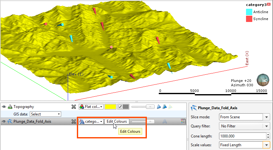
Another way of displaying planar structural data is to display the categories as different colours:
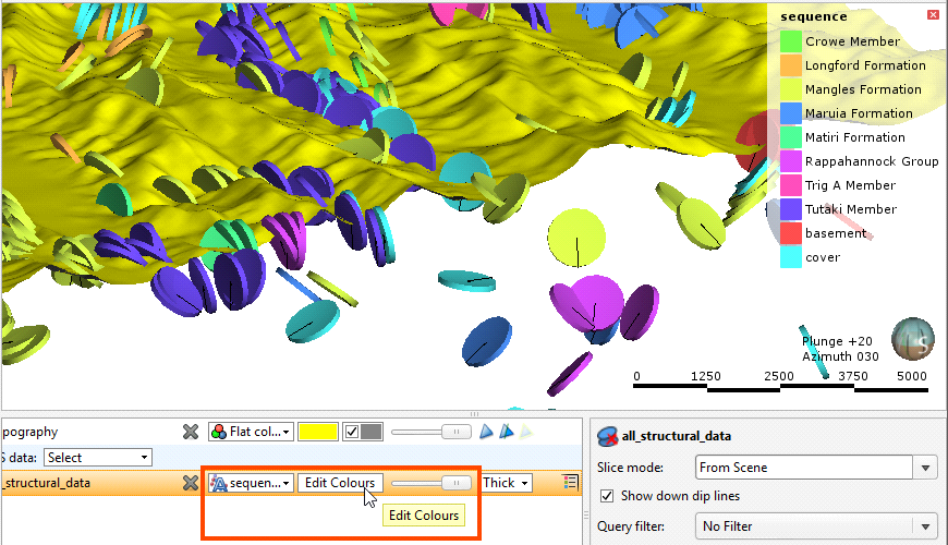
You can change the colours used to display the different categories by clicking on Edit Colours in the shape list. In the window that appears, click on the colour chip for each category and change it as described in Single Colour Display.
To set multiple categories to a single colour, use the Shift or Ctrl keys to select the colour chips you wish to change, then click on one of the colour chips. The colour changes you make will be made to all selected categories.
The categories displayed can also be filtered by other columns in the data table, as described in Filtering Data Using Values and Categories.
In the scene below, lineations are displayed using the Flat colour option in green:
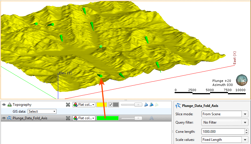
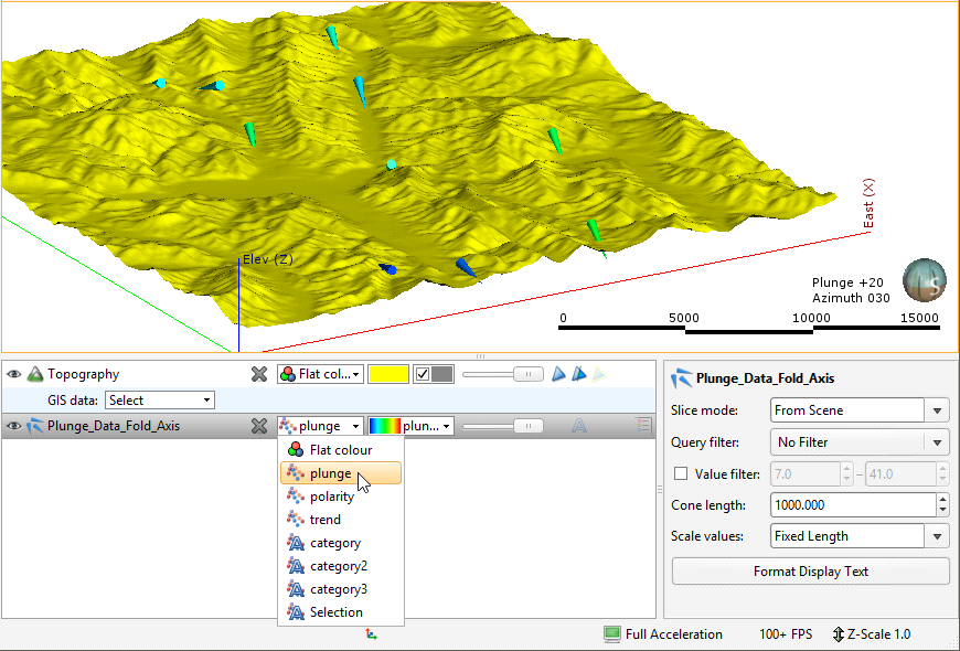
Click the colour chip to change the colour used to display the cones in the shape list or select one of the table’s columns:
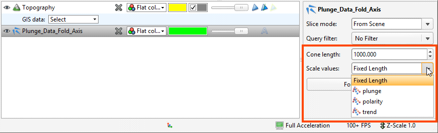
The length of the cones displayed in the scene is set in the properties panel. This can be a Fixed Length, defined by the Cone length setting, or it can be scaled using the values from one of the table’s columns:
Another way of displaying lineations is to display the categories as different colours:
You can change the colours used to display the different categories by clicking on Edit Colours in the shape list. In the window that appears, click on the colour chip for each category and change it as described in Single Colour Display.
To set multiple categories to a single colour, use the Shift or Ctrl keys to select the colour chips you wish to change, then click on one of the colour chips. The colour changes you make will be made to all selected categories.
The categories displayed can also be filtered by other columns in the data table, as described in Filtering Data Using Values and Categories.
Viewing Statistics on Structural Data
To view statistics on structural data and lineations, right-click on a table and select Statistics. The following options are available:
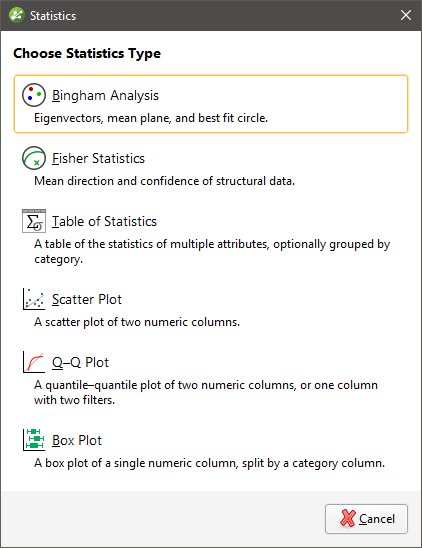
See the Analysing Data topic for more information on each option:
Bingham Analysis
The Bingham Analysis option shows the value, trend and plunge for each of the eigenvectors, along with the Bingham mean plane and best-fit great circle:
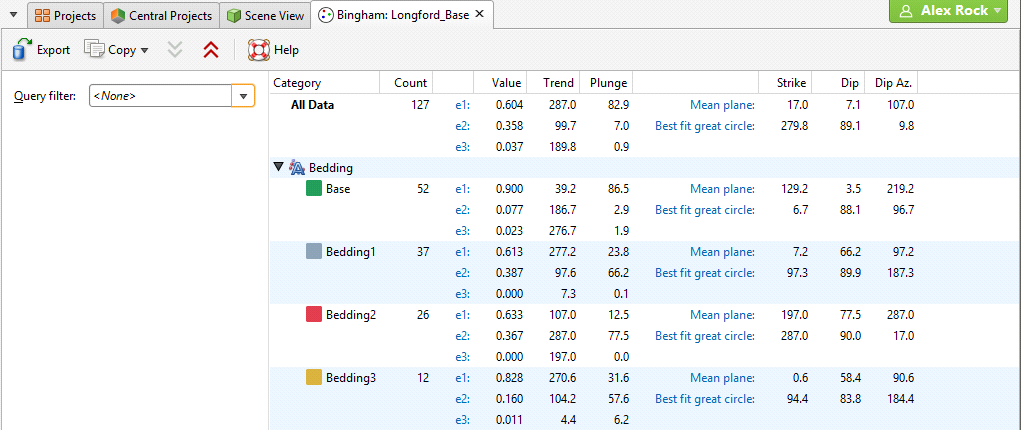
You can select specific rows and copy them to the clipboard or copy all data to the clipboard. You can also export the data in *.csv format.
Fisher Statistics
The Fisher Statistics option shows the Fisher mean plane and confidence for the data in the selected table:
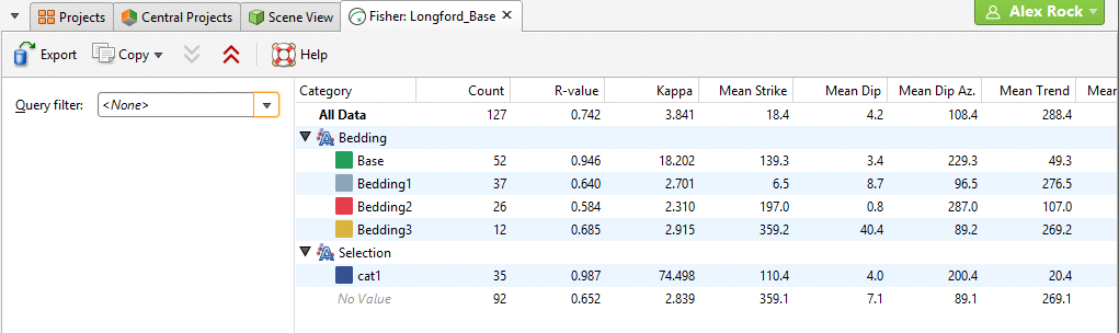
You can select specific rows and copy them to the clipboard or copy all data to the clipboard. You can also export the data in *.csv format.
Assigning Structural Data to Categories
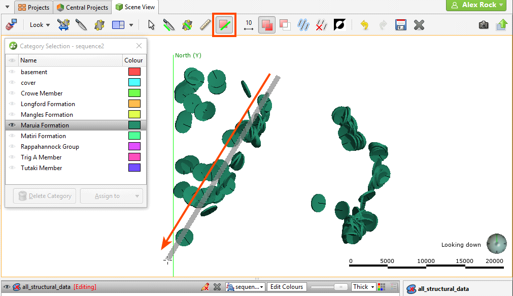
There are two ways to initiate structural data selection: from the data object in the project tree/shape list and from a stereonet. The advantage of initiating structural data selection from a stereonet is that the data will be displayed both on the stereonet and in the scene window. This provides the most flexibility for analysing what data belongs to what category. See Selecting Data in the Stereonet and Using the Scene Window With the Stereonet for more information.
If you wish to assign planar structural data points or lineations to categories, right-click on the data table in the project tree and select New Category Selection. First, select the Source Column. If you select an existing column as the Source Column, you can assign selected data points to existing categories or create new categories. If you select <None> for the Source Column, you will have to define each category manually.
Select points by clicking on the Select points tool (![]() ), then drawing over those points in the scene:
), then drawing over those points in the scene:
Once you have selected points, you can assign them to existing categories or create new ones. To create a new category, click on the Assign to > Create New Category button:
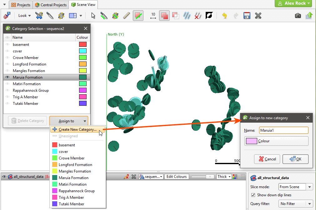
Enter a name for the new category and click OK.
When you have finished selecting points and adding them to categories, close the Category Selection window to close the editor.
Editing the Orientation of Planar Structural Data
If you need to edit the orientation of planar structural data points, you can do so in two ways:
- Edit the data in the table directly by double-clicking on the structural data table in the project tree. See Working With Data Tables.
- Edit the structural data orientation in the scene.
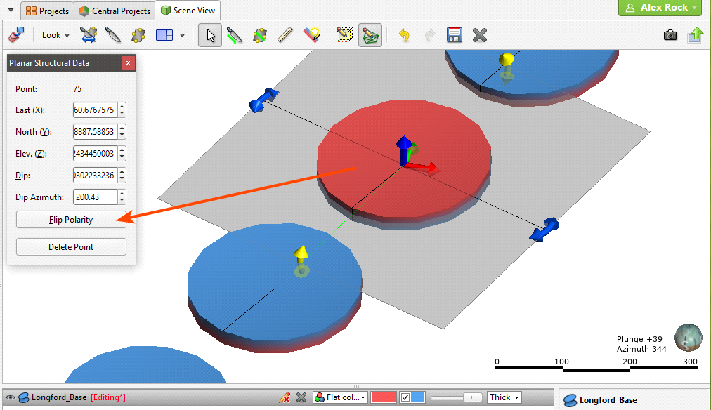
To edit the structural data in the scene, right-click on the table in the project tree and select Edit Orientation in Scene. If the table is displayed in the scene, in the shape list, click on the Edit button (![]() ). The Planar Structural Data window will appear in the scene, together with controls for editing the data points. To edit a data point, click on it. Information about the selected point will be displayed in the Planar Structural Data window, together with controls in the scene you can use to adjust the point:
). The Planar Structural Data window will appear in the scene, together with controls for editing the data points. To edit a data point, click on it. Information about the selected point will be displayed in the Planar Structural Data window, together with controls in the scene you can use to adjust the point:
You can also add new data points in the same manner described in Creating New Planar Structural Data Tables.
Declustering Planar Structural Data
If a planar structural data table contains multiple duplicate or near-duplicate measurements, you can create a declustered structural data set that will make the table easier to work with. Declustering is intended to work with large, machine-collected data sets rather than smaller sets that might be edited manually.
Declustering preserves the original data table and creates the set as a “filter” by applying two parameters: the Spatial search radius and the Angular tolerance.
- The Spatial search radius determines the size of the declustering space. All points inside the Spatial search radius are compared searching for duplicates.
- The Angular tolerance measures whether points have the same or similar orientation. The orientation of all points inside the Spatial search radius is measured and the mean taken. If a point’s orientation is less than the Angular tolerance from the mean, then the point is regarded as a duplicate. The point that is retained is the one that is closest to the mean.
When a structural data set has a numeric column that gives some indication of the measurement’s uncertainty, this column can be used to prioritise values. Select the Priority column and set how the values should be handled.
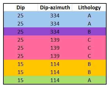
Another factor in declustering the points is the category columns selected. When you choose multiple category columns, all criteria must match for points to be regarded as duplicates. What this means is that points will be kept if they have different category values in just one column, even if they meet the criteria for duplicates established by the Spatial search radius and the Angular tolerance and match in other columns. For example, in this table, assume that applying the Spatial search radius and the Angular tolerance parameters without using the Lithology category results in three points. However, including the Lithology column results in five points, indicated by the colours:
The more columns you select, the lower the likelihood that points will be regarded as duplicate.
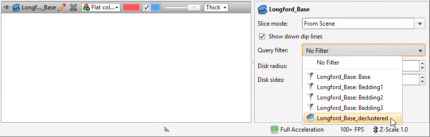
The declustered set can be used like an ordinary structural data table. However, it is a filter on a planar structural data table and can be used as such when the parent table is displayed in the scene. For example, here the filters available for the planar structural data table include the query filters (![]() ) defined for the table as well as the declustered set (
) defined for the table as well as the declustered set (![]() ):
):
To create a declustered structural data set, right-click on the Structural Modelling folder and select New Declustered Structural Data. Select the source data table and a query filter, if required. Set the parameters and the columns you wish to use, then click OK. The declustered set will be added to the Structural Modelling folder.
Edit the set by right-clicking on it in the project tree and selecting Edit Declustered Structural Data.
Setting Elevation for Structural Data
You can set the elevation for planar structural data points or lineations by projecting the data onto a surface. Any elevation data in the data table will be overwritten by the elevation values from the selected surface.
To set the elevation for planar structural data points or lineations, right-click on the table in the project tree and select Set Elevation. The Set Elevation from Surface window will appear:
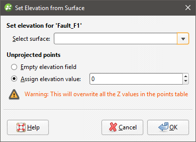
Select from the surfaces available in the project.
Unprojected points are data points that do not vertically intersect the selected surface. There are two options for handling these points:
- Leave the elevation field empty.
- Assign a fixed elevation value.
Click OK to set elevation values.
Estimating Planar Structural Data
You can generate a set of planar structural measurements from points, polylines and GIS lines. To do this, right-click on the points or lines object in the project tree and select Estimate Structural Data. In the window that appears, enter a name for the structural data table, then click OK. The new structural data table will appear in the project tree and you can view and edit it as described in Displaying Structural Data and Editing the Orientation of Planar Structural Data.
Got a question? Visit the Seequent forums or Seequent support