Grid Data - Multi-trend

Gridding refers to the process of interpolating data onto an equally spaced “grid” of cells in a specified coordinate system. For an introduction to gridding and a summary of the different gridding methods click here.

Multi-trend Gridding

The multi-trend gridding method uses the NSI gridding algorithm¹ to grid a database channel.

To perform multi-trend gridding, you must supply a data channel, an output grid name, and optionally the final grid cell size. In addition, you have the ability to:

• filter out values from the gridding process.

• specify an initial interpolation grid cell size.

• define a blanking distance (for removing values beyond a certain distance).

• specify the maximum number of iterations to allow.

• adjust the trend direction and the smoothing factor to reveal distinctive or more predominant linear trends.

Use the Grid Data option from the Grid and Image > Gridding menu to grid data using the multi-trend gridding algorithm and generate a grid file (*.grd).

Multi-trend – Gridding Options

Data to grid	Select the database channel to grid. To specify an array element, append to the channel array name the element index in square brackets. For example, Chan[1] would indicate the second element of the array channel "Chan". Script Parameter: NSI_GRIDDING.CHANNEL
Output grid	Provide the name of the output grid file. This field is auto populated based on the active database and the selected channel to grid; however, you can override the default. The default output grid format is selected automatically as the output file type. The type can be controlled using the browse dialog, which is accessible from the [...] button. Script Parameter: NSI_GRIDDING.GRID
Gridding method	The current gridding method is displayed. Script Parameter: GRIDDING_TOOL.METHOD [Multi-trend: 5]
Cell size	Specify a (final) cell size (in data units) for the output grid. This field is auto-populated with the calculated default grid cell size and rounded to the nearest ten or hundred: Default grid cell size The grid cell size (the distance between grid points in the X and Y directions) should normally be ¼ to ½ of the line separation or the nominal data sample interval. If not specified, the data points are assumed to be evenly distributed and the default cell size will be set to: Where: The final cell size must be greater than or equal to the starting cell size. See the Application Notes below for more details on adjusting the grid cell size. Script Parameter: NSI_GRIDDING.FINAL_CELL_SIZE
Extents and Data
Spatial Extents
Grid extents (X min, Y min, X max, Y max)	Define the spatial limits of the area to be gridded. By default, these fields are set to the full extents of the current X & Y channels of the active database in order to include all the data in the database: X min, Y min: the ground coordinates of the first grid point at the bottom left corner of the rectangular grid area (by default, the minimum limits of the input data file are used). X max, Y max: the ground coordinates of the last grid point at the top right corner of the rectangular grid area (by default, the maximum limits of the input data file are used). To grid a subset of the data, enter the limits of the bounding rectangle, or press the Draw Extents button to interactively define the boundary extents – the output grid coverage will extend to these limits. Script Parameter: NSI_GRIDDING.XY
[Draw Extents]	Press this button to interactively define the grid boundary extents: in the Grid Preview pane, use the mouse to click & drag to draw a box, then release the mouse cursor to accept the final size of the box. The X & Y values will be updated in the Grid extents fields, and the preview window will be refreshed to show the newly defined extents. You can draw the box in any of the four possible ways (e.g., from bottom left to top right).
[Reset Extents]	Press this button to reset the grid extents to the initial state of defaults for the active database. The Grid Preview pane (when Auto-refresh is enabled) will be updated to reflect the change; however, the zoomed state (in/out) of the grid preview will not be affected.
Cells to extend beyond data	This is the number of grid cells to extend beyond the outside limits of the data. If the default is preserved (set to zero), the grid extents are limited to just overlapping the most extreme data value locations in X and Y. Set this to a number greater than zero to allow the grid to be extrapolated beyond the data edges. The actual extrapolation distance is limited by the Blanking distance value, and cells extended beyond this distance will remain dummies in the output grid. Do not use this parameter in place of the blanking distance in order to fill interior regions of the grid, as results are generally poorer than using the blanking distance. This is because the blanking distance measures the true radial distance between a given location and the nearest data point, while the "cells to extend" is measured only in X or in Y. The blanking distance is a true distance and the "cells to extend" is the number of cells, so you must multiply by the actual cell size to compare the two. Script Parameter: NSI_GRIDDING.CELLS_TO_EXTEND (Default: 0)
Data Filtering
Mask channel	Select a channel from the drop-down list to act as a mask. Only database channels that have the class property set as "MASK" are listed. Additionally, string channels and channels with array size greater than 1 are omitted from the list. The data values in the selected Data to grid channel with corresponding dummy (*) values in the Mask channel will not be used in the gridding process. The X & Y values will be updated in the Grid extents fields to reflect the masked data, and the generated masked grid (with the correct extents) will be automatically rendered in the Grid Preview window (the Auto-refresh option must be selected).  Script Parameter: NSI_GRIDDING.MASK_CHANNEL
Interpolation
Multi-trend
Starting cell size	Specify the initial interpolation grid cell size (in data units). By default, Starting cell size is set to Cell size/2. Script Parameter: NSI_GRIDDING.CELL_SIZE
Blanking distance	Enter the interpolation distance. All grid cells within this distance of valid surveyed data will be evaluated; grid cells farther than this value from a valid point will be set to dummies in the output grid. This parameter has a dual function, as it is also used as the search radius to find linear trends. As a result, it should be set to exceed your line spacing and set subject to the expected lengths of the linear features to join. By default, Blanking distance is set to Starting cell size x 5. Script Parameter: NSI_GRIDDING.INTERP_DISTANCE
Max iterations	Enter the maximum number of iterations (at each level of grid refinement) after which the gridding process stops. The default is set to 50. Increase this value to produce a grid that honours the survey data more closely. Script Parameter: NSI_GRIDDING.MAX_ITER
Automatic stopping criteria	Select this field to automatically stop the gridding process before reaching the specified maximum number of iterations. The iterations will stop if the average difference between the current and previous solutions continues converging over three consecutive iterations. Script Parameter: NSI_GRIDDING.AUTO_STOP [0: No, 1: Yes (default)]
Trending factor	Select a value between 0 and 100. The higher the trending factor, the smoother the lineaments will be. The default is set to 50. Trending factor will default to 50 if the entry is left blank. Script Parameter: NSI_GRIDDING.TRENDING_FACTOR
Theta	This is the increment in degrees by which to rotate the trend direction, in order to have an adequate number of survey points within the search radius for calculating the grid value at the centre of the search circle. The trend direction is rotated in the CW (clockwise) direction. The default is set to 10. See the Application Notes below for more information. Script Parameter: NSI_GRIDDING.THETA
Multi-smooth factor	Select a value between 0 and 100. The lower the smoothing factor, the more unique trending directions are allowed. By default it is set to 0, which will find linear features in any given azimuth direction. Increasing this value will focus on the predominant linear trends. Modify this setting if high-frequency features (small, isolated discrepancies) appear too frequently, and they are not minimized by the subsampling process of the starting cell size to the final cell size. Script Parameter: NSI_GRIDDING.MULTI_SMOOTH
[Restore Defaults]	This button remains disabled until any of the fields default values are changed. Press the button to reset the gridding parameters to the initial state of defaults for the active database. When Restore Defaults is clicked: The following parameters are reset to their default values: The cell size value All the parameters on both the Extents and Data and Interpolation tabs Only the parameters for the current gridding method are affected. The following parameters are not reset: The data to grid selection The output grid file name The gridding method The Grid Preview (with Auto-refresh enabled) and Variogram panes will be updated to reflect any parameters changes; however, the zoomed state (in/out) of the grid preview will not be affected.

Application Notes

Adjusting the Cell Size

Grid cell size should not be much less than half the nominal data point interval found in the areas of interest. A smaller cell size will more accurately fit the data points, but if the data contain errors this may not be desirable; it also means longer processing time and a larger output data size. A small cell size may also require a reduction in the iteration tolerance and an increase in the number of iterations to achieve an acceptable result. If the cell size chosen is smaller than the average data point density, then there will be many gaps in the output grid.

If the data is to be contoured (we recommend 2 mm or 1/10 inch at plot scale for contouring), specify a smaller cell size and a larger desampling factor or regrid the grid using bi-directional gridding.

With a larger cell size, the gridding algorithm averages more data points per grid node, thus the data appears smoother. However, increasing the cell size further is likely to introduce adverse results. It may dilute grid patterns that correspond to real geological features, thus obscuring real features. While dealing with large datasets, be aware of the trade-off between the processing accuracy and processing time, as well as the data storage requirements.

Final Grid Cell Size

Once the interpolation is complete, the method will subsample the entire grid up to the larger, more appropriate,final grid cell size. For strong linear features, the smaller cell size can assist in making the features smoother due to the effect of subsampling. However, a small cell size must be used with caution as it can often remove weaker linear features; they will now have “farther” to trend when connecting lineaments found in the real data cells [T. Naprstek].

Theta

To explain the effect of Theta, we refer you to Figure 1 below. In this schematic, the observed data is in cyan and the point being evaluated is indicated in light green. The observed values used for the evaluation reside within the search radius (purple circle) around the green cell. The original trend direction, determined by the structure tensor, is shown by the green solid line.

If the trend line does not intercept real data within the search radius, the trend is shifted by Theta (Θ₁ on the schematic) to the direction indicated by the red solid line, and the search for real data is attempted again. In the illustration, the solid red line intercepts valid cells on one side, and the general trend is slightly shifted and honoured.

However, if Theta is large (Θ₂ on the schematic), data along the dashed red line would be analyzed. This may deviate too much from the desired linear trend and connect trends that don’t belong together.

It is recommended to set the angle relatively small to stay within the general trend direction determined by the structure. Note that a very small angle may increase the number of iterations and make the gridding process slower.

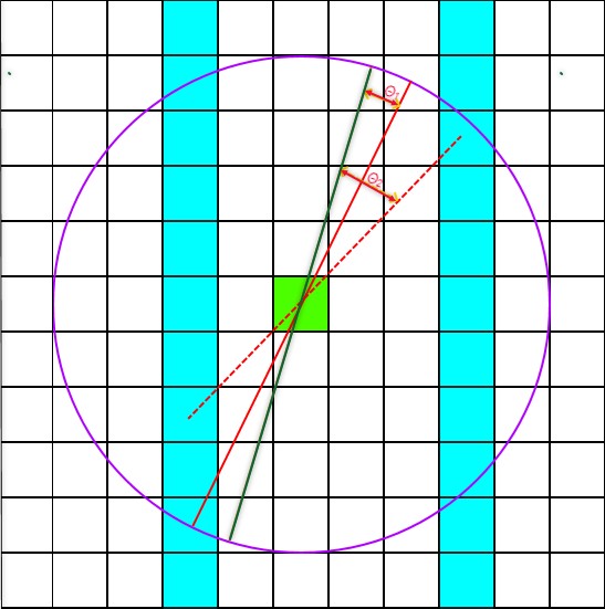
Figure 1: The blue cells contain real data; the green cell is the cell being evaluated; the purple circle is the search radius.

Spatial Smoothing

In the case where an extremely small cell size (< 0.1) is used, the partial derivatives calculated during the Taylor Interpolation step will "explode", meaning that even after one or two iterations they become so large as to be computationally inefficient. In this case, spatial smoothing is turned off, and the partial derivatives are removed from this step effectively reducing it to a more simplistic smoothing operator. This has the effect of reducing the amount of linear structure in the output grid in particular in areas where lineaments are "weak" (low amplitude).

Such a small cell size generally only occurs when input data have geographic (latitude and longitude) coordinates, which have ground units of degrees. The implication of this is that if your data is in geographic coordinates, but you want to maximise the linear structure in the output grid, then you should reproject your data into a projected coordinate system before using the multi-trend gridding method.

¹ Acknowledgment