
Gridding Data Methods - Overview and Comparison
What is gridding and how does it work?
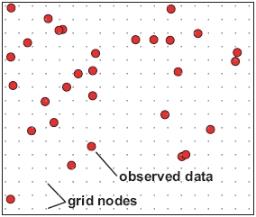
When dealing with two-dimensional data, it is useful to represent the data by determining its value at points located equally far apart at the nodes of a grid, as shown in the following figure:
Data in a grid format can have a number of two-dimensional processes, such as image processing, computer contouring or two-dimensional filtering, applied to it.
The values at the grid nodes can be determined by taking readings at the node locations. However, in practice this is seldom convenient. It is more likely to have data that has been collected at random locations, or which has been collected at a relatively high sample density along more widely separated parallel lines. Such raw data is commonly referred to as XYZ data, because each data point has a (X,Y) location and one or more measured (Z) values.
Gridding data is the process of spatial interpolation. The process of gridding takes point (XYZ) data and interpolates the readings to determine the values at the nodes of a grid in between the data points. The resulting interpolated data set is known as a grid.
The table below provides a summary of the different gridding methods you can use to grid your data as well as fundamental gridding concepts. A comparison between some of the most common gridding methods is outlined as well.
Overview of Gridding Data Methods
Gridding method |
What does it do and when to use it |
|
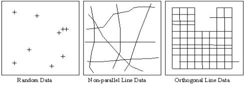
The minimum curvature method interpolates the data by fitting a two-dimensional surface to the raw XYZ data in such a way that the curvature of the surface is minimized. This approach to fit a minimum curvature surface to the data points uses a method similar to that described by Briggs (1974) and Swain (1976) and is ideal when the surface is expected to be relatively smooth or continuous between data points. It is best used when data is randomly distributed, sampled along arbitrary lines, or if you want to include tie lines. The figure below illustrates the types of data distribution: Data distribution suitable for minimum curvature gridding If the data is relatively smooth between sample points or survey lines, minimum curvature gridding should be used. If the data may be variable between sample locations, or it is known to be statistical in nature (such as geochemical data), poorly sampled or clustered, use the kriging method.
Minimum curvature gridding first estimates grid values at the nodes of a coarse grid (usually 8 times the final grid cell size). This estimate is based upon the inverse distance average of the actual data within a specified search radius. If there is no data within that radius, the average of all data points in the grid is used. An iterative method is then employed to adjust the grid to fit the actual data points nearest the coarse grid nodes. A very important parameter in the minimum curvature gridding process is the number of iterations used to fit the surface at each step. The greater the number of iterations, the closer the final surface will be to a true minimum curvature surface. However, the processing time is proportional to the number of iterations. Minimum curvature gridding stops iterating when:
By default, these limits are 100 iterations and 99% of points within 1% of the data range.
|
|
|
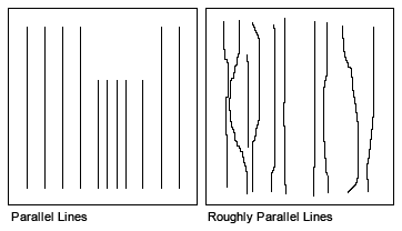
The Bi-directional gridding method (BIGRID) is a numerical technique for gridding parallel survey lines or roughly parallel lines, as illustrated in the figure below.
Data distribution suitable for bi-directional gridding BIGRID is the only gridding method that can take advantage of a strong line-to-line correlation of otherwise narrow features in line data; it joins narrow features that extend from line to line perpendicular to the line direction. BIGRID is ideal in these situations, especially if there is a high sample density down the lines relative to the line separation. The method cannot be applied to randomly distributed XYZ data. Line data that is measured along orthogonal lines is also not well suited to BIGRID: the method does not use tie lines; if data on the tie lines is important, minimum curvature or kriging should be used. This gridding method uses linear, minimum curvature, or Akima splines to interpolate grid nodes between lines in the direction of the overall trend of the data, which is usually perpendicular to the survey lines. In addition to trend enhancement, bi-directional gridding allows the method of interpolation to be selected independently for the down-line and across-line directions. Geological trends in the data can be emphasized by the appropriate orientation of the grid so that the across-line interpolation is in the direction of the trend. BIGRID can be 10 to 100 times faster than the minimum curvature gridding (RANGRID), and up to 1000 times faster than kriging (KRIGRID). BIGRID has the following strengths and features:
|
|
|
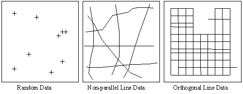
This statistical gridding method interpolates the data using the kriging (or Kriging) technique to determine the most probable value at each grid node based on the located data provided and using a statistical analysis of the entire dataset. Kriging is a geostatistical gridding technique for random data, non-parallel line data or orthogonal line data (as illustrated in the figure below). Use the Kriging method if the data is variable between sample locations, known to be statistical in nature, or poorly sampled or clustered. Kriging is ideally suited to geochemical or other geological sample-based data; it is rarely used with geophysical data, which tends to follow a natural smooth surface. The figure below illustrates these types of data: Data distribution suitable for kriging Based upon kriging statistics, the kriging (KRIGRID) method is also able to estimate the error of the data at each grid node and to produce an error grid. This error grid gives an indication of the degree of confidence at each grid node. Oasis montaj supports ordinary Kriging as well as universal Kriging. Universal kriging differs from ordinary kriging in that it enables the data to contain a regional trend. For more details check the Kriging Theory, and for a more in-depth understanding of the geostatistical analysis and kriging refer to Journel and Huijbregts [3]. Kriging has the following capabilities:
|
|
|
Inverse Distance Weighted (IDW) Gridding |
The Inverse Distance Weighting (IDW) algorithm is a moving-average interpolation algorithm that is usually applied to highly variable data. For certain types of data (e.g., soil geochemistry, surface/groundwater chemistry) it is possible to return to an existing measurement site and record a measurement that is statistically different from the original, but within the general trend of all measurements within the area. In this case it is not usually desirable to honour local data minima or maxima, but instead to look at a moving average of surrounding data points and estimate local trends. IDW calculates a value for each grid node by examining surrounding data points that lie within a user-defined search radius. The node value is calculated by averaging the weighted sum of all the points, where the weighting inversely corresponds to distance from the grid node. |
|
Direct Gridding |
The Direct Gridding method creates a grid from highly sampled data without using any interpolation and provides a quick gridded view of the datasets. This method is intended for use with over-sampled datasets such as LiDAR. It is an adequate method for oversampled data, and it is a fast method since it bypasses the splining and iterative calculations of the minimum curvature surface; however, it does not compensate for the under-sampling of the data. |
|
TIN Gridding (TINNING) |
The TIN gridding method (TINNING) requires one data point for each (X, Y) data location in the database. Tinning provides the ability to sum or average duplicate samples - data that have multiple Z values at single point locations. (Note that, when Z values are included in the (*.tin) file, only data point locations with non-dummy Z values are included.) The ability to create a TIN (Triangular Irregular Network) and to use this TIN to grid data using the "Nearest Neighbour", "Linear", and the "Natural Neighbours" methods has been added to the Oasis montaj environment. The TIN is created from a set of spatial data using the public domain Sweepline algorithm implemented by Steven Fortune of Bell Laboratories (Fortune, S 1987). The TINDB GX applies the Sweepline algorithm to the X, Y (Z-optional) data values in a Geosoft Database (*.gdb) to create a binary TIN (*.tin) file. When Z values are included in the (*.tin) file, a TIN grid can be created using the TINGRID GX. The TINGRID GX can create a grid using the Linear, Nearest Neighbour, or Natural Neighbour algorithm [Sambridge et al, 1995]4, to the Z values in the (*.tin) file to create a grid. There are three methods available for gridding your TIN:
Oasis montaj Tinning provides a number of ways of visualizing the TIN, including the ability to: |
Other Gridding Options:
-
Gridding from a Control File:
What method should I use: BIGRID, RANGRID, KRIGRID or TINNING?
Use bi-directional gridding (BIGRID) if the data is collected along lines that are roughly parallel, as in the following examples:
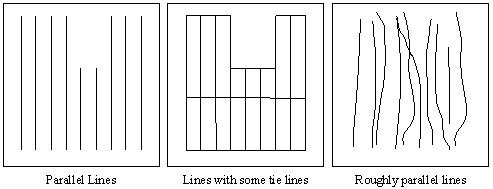
BIGRID is ideal in these situations, especially if there is a high sample density down the lines relative to the line separation. Furthermore, BIGRID is able to join narrow features that extend from line to line perpendicular to the line direction.
BIGRID is not able to use the tie lines, as shown in the middle example, because of the way the gridding algorithm works. If the data on the tie lines is important, minimum curvature gridding (RANGRID) or kriging (KRIGRID) should be used.
Based on very general criteria, Minimum curvature, Tinning, Inverse Distance Weighting and Kriging are all optimal methods for statistical data such as that from geochemical surveys, based on your data. Since geochemical data are statistical in nature and have a high range from sample to sample, it may also be appropriate to reduce the range of data through standard processing (i.e. application of a logarithmic transform).
Use RANGRID, KRIGRID or TIN Gridding (TINNING) when the XYZ data is not sampled along lines that run in roughly the same direction. Such data are often called random, because they give a random appearance when the data locations are plotted. Also, line data with survey lines that are orthogonal (or have random directions) should be gridded with RANGRID, KRIGRID or TINNING. The following figure illustrates these types of data:
If the data is relatively smooth between sample points or survey lines, then RANGRID should be used.
Use KRIGRID if the data:
-
is variable between sample locations.
-
is known to be statistical in nature (such as geochemical data).
-
is poorly sampled.
-
is clustered.
Use TINNING if the data:
-
is variable between sample locations.
-
is highly irregular in distribution.
References:
- [1] I. C. Briggs, "Machine contouring using minimum curvature", Geophysics, vol. 39, no. 1 (1974), pp. 39-48.
DOI: https://doi.org/10.1190/1.1440410. - [2] C. J. Swain, "A FORTRAN IV program for interpolating irregularly spaced data using the difference equations for minimum curvature", Computers and Geosciences, vol. 1, no. 4 (1976), pp. 231-240.
DOI: https://doi.org/10.1016/0098-3004(76)90071-6. - [3] C. A.G. Journel and Ch.J. Huijbregts, Mining Geostatistics (London: Academic Press, 1978).
- [4] Malcolm Sambridge, Jean Braun, Herbert McQueen, "Geophysical parametrization and interpolation of irregular data using natural neighbours", Geophysical Journal International , vol. 122, no. 3 (December 1995), pp. 837-857.
DOI: https://doi.org/10.1111/j.1365-246X.1995.tb06841.x.
Got a question? Visit the Seequent forums or Seequent support
© 2023 Seequent, The Bentley Subsurface Company
Privacy | Terms of Use