Grid Data - Variogram Tab

The Variogram tab is available when the current gridding method in the Grid Data tool is "Kriging". Click on this tab to view a plot of the variogram of the data generated based on the current variogram model and parameters. Evaluate the data and use the left pane of the Grid Data tool to select the optimal variogram model and parameters – press the Update button located in the Variogram section of the Interpolation tab, and the variogram will be regenerated based on the adjusted variogram parameters.

Selecting the optimal variogram model is key to obtaining high-quality results for the output grid. When the variogram displays a better fit to the observed data, you are ready to grid the data using the model created. The calculated variogram will be placed in the output variogram file specified under the Interpolation tab.

The Variogram Window

Kriging is a multistep process; it includes exploratory statistical analysis of the data and variogram modeling. The approach is to first calculate a variogram of the data, which shows the correlation of the data as a function of distance. Simply speaking, the further apart the data points become, the greater the variation between the points and less correlation we expect between points. The variogram shows this phenomena for a given dataset, and based on the variogram, you are able to select a model that best defines the variance of the data.

The example below illustrates a variogram of data generated based on the spherical model and the intelligent calculated defaults for the variogram model parameters:

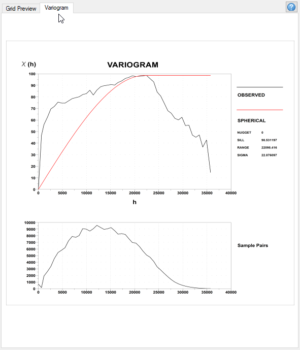
The variogram (in fact this is the semi-variogram, but we call it variogram for brevity) shows the correlation (semivariance) of the data as a function of the distance away from the sampling point. Ideally, the red curve representing the variogram model should match the black line representing the observed data. Normally, the variogram reaches a point (sill value) at which the semi-variance (variogram) plateaus. The corresponding h value is called the range value – beyond this distance there is no similarity in samples. At the right end of the variogram, the variability may appear to decrease, but this is usually the result of too few pairs of samples for the statistics to be valid.

The sample pairs are plotted below the variogram. The plot shows how many sets of samples occur within specified distances of each other – this curve may help you to refine your variogram in the selection of the data points used to visualize your model curve. In the illustration above, most of the data occurs within ~ 12 000 m, and data beyond this point should not be given as high an emphasis when building the variogram.

Selecting a model and parameters is the toughest part of your kriging decision and requires considerable experience. Kriging is suitable for clustered data in which clusters are characterized by a relatively large number of samples and may be widely spaced. Typically, you would use kriging to grid data within clusters accurately and then truncate the model between clusters so that clusters do not affect the gridding of neighbouring clusters. Examine the error grid to verify that data integrity is maintained both within and between clusters. Adjust the variogram parameters and then create the gridded data. Note that any parameters that are not defined will be calculated from the data based on a fitting algorithm for each model. You will typically have to adjust the automatic parameters manually to better fit your own data model.

Variogram Models

The variogram of the data shows the anticipated increase in variability as h increases and is calculated using the expression:

The function shows the correlation of observed data as a function of distance between points.

Kriging requires a model of the observed variogram to determine the weighting factors used in the kriging matrix. Although observed variograms can appear quite noisy, it is important that the model used is both smooth and has increasing variability with increasing h; the statistical accuracy of kriged results is related to how close the model is to the observed variogram.

Kriging Models

There are four types of variograms you can generate in the system based on the models below:

Power Model

The linear power model (n = 1) is the default model used in kriging (KRIGRID). Only the power model can be determined automatically by KRIGRID - all other models require you to enter the model parameters. KRIGRID uses least square fitting to determine the slope of the linear model for a line that starts at (0,0). If this is unacceptable, use the control file parameter "nugget" to set the intercept, and the parameter "range" to define the slope.

The power model follows the expression:

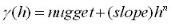
As a guideline, the power (or linear) model can be acceptable when the nominal group of nearest and second-nearest data points are well within the area of the model where the model line is still close to the observed variogram. This is seldom the case for clustered data.

Spherical Model

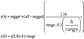
The spherical model is the most common used in geological situations. To use the spherical model, you must first plot out the variogram of the data you are working with and determine the optimum range, nugget and sill.

The spherical model has the following expression:

Gaussian Model

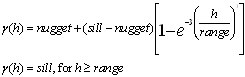
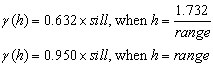
To use the Gaussian model, you must first plot out the variogram of the data you are working with and determine the optimum range, nugget and sill. With this model, the sill is actually never reached and at the range of the model is 5% less than the sill.

The Gaussian model has the following expression:

Where:

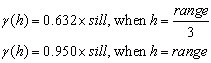
Exponential Model

To use the exponential model, you must first plot out the variogram of the data you are working with and determine the optimum range, nugget, and sill. As with the Gaussian model, the sill is actually never reached. At the range, the model is 5% less than the sill.

The exponential model follows the expression:

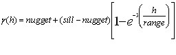
Where:

The Variogram File Format

The kriging method (KRIGRID) will write out the variogram of the data in the (*.var) file specified.

The file is a standard Geosoft data file (ASCII text) that begins with comment lines containing information about the variogram model, in this case a spherical model . The model parameters are listed (model, nugget, sill, and range), together with SIGMA, which is the RMS difference between the variogram model and the observed variogram. The data columns contain the distance between samples (VH), the observed variogram (VG), the modelled variogram (VM), the number of points averaged to calculate the variogram (NP), and an index (I).